


Overview
Source: Alexander S Rattner, Sanjay Adhikari, and Mahdi Nabil; Department of Mechanical and Nuclear Engineering, The Pennsylvania State University, University Park, PA
Controlled heating followed by rapid cooling is an important element of many materials processing applications. This heat-treating procedure can increase material hardness, which is important for cutting tools or surfaces in high wear environments. The rapid cooling stage is called quenching, and is often performed by immersing materials in a fluid bath (often water or oil). Quenching heat transfer can occur due to forced convection - when the action of rapidly moving material through coolant drives the heat transfer process, and due to free convection - when the reduced density of hot fluid near the material surface causes buoyancy-driven circulation and heat transfer. At high material temperatures, the coolant can boil, leading to increased heat transfer effectiveness. However, when extremely hot materials are quenched, they can be blanketed in relatively low thermal conductivity coolant vapor, leading to poor heat transfer.
In this experiment, quenching heat transfer will be measured for a heated copper cylinder, which is representative of small heat-treated parts. The transient sample temperature profile will be measured during quenching and compared with theoretical results for free convection heat transfer. Boiling phenomena will also be investigated qualitatively.
Principles
The process of quenching heat transfer is fundamentally transient. In general, the temperature distribution can vary in space and time inside a cooled material sample. However, if internal conduction thermal resistance is small compared with external thermal resistance from the sample surface to the surrounding fluid (convection), the sample can be assumed to have nearly uniform temperature at any instant, simplifying analysis. This condition can be expressed in terms of the Biot number (Bi), which compares internal conduction resistance to external convection resistance. Generally, when Bi < 0.1, internal heat transfer resistance can be assumed negligible compared to external heat transfer resistance.
 (1)
(1)
Here, h is the external convection coefficient, ks is the thermal conductivity of the sample, and Lc is a characteristic length scale of the sample. h can be predicted using heat transfer models and curve fits published in the literature for different conditions and fluids. In this experiment, h will be measured and compared with results predicted with published models (see Representative Results section).
For the copper cylinder considered here (k = 390 W m-1 K-1, diameter D = 9.53 mm, length L = 24 mm), the characteristic length scale is D/2 = 4.8 mm. Assuming a maximum convection coefficient of h = 5000 W m-2 K-1, the peak Biot number would be 0.06. As this number is small (< 0.1), it is reasonable to assume that internal conduction resistances are negligible, and the sample has uniform temperature. At higher Bi values, a more complicated analysis is needed that accounts for temperature variation in the material.
Assuming a uniform-temperature sample, the heat transfer rate can be modeled by balancing internal energy loss from the sample with the convective heat removal rate from Newton's law of cooling. This approach is called a lumped capacitance analysis.
 (2)
(2)
Here, m is the sample mass (15 g), c is the specific heat of the sample material (385 J kg-1 K-1 for copper), Ts is the sample temperature, As is the sample surface area (8.6 × 10⁻⁴ m2), and  is the surrounding fluid temperature.
To predict the cooling rate (dTs/dt) during quenching, the convection coefficient (h) must also be predicted. If the sample is below the fluid boiling temperature and held stationary in a pool of coolant, then heat is primarily removed by free convection. In this mode, circulation and cooling is produced by the buoyancy-driven rising of heated fluid near the sample. Greater sample-to-fluid temperature differences result in increased circulation rates.
If the sample temperature is above the boiling point, vapor can be generated at the surface, resulting in significantly higher cooling rates. During boiling, vapor bubbles form and grow from small imperfections (nucleation sites) on the hot surface. At higher surface temperatures, more nucleation sites become active, resulting in greater convection coefficients and higher heat transfer rates. However, at very high temperatures, the relatively low conductivity vapor cannot be removed fast enough. This results in the boiling crisis, in which the surface cooling is limited due to vapor insulation, reducing the heat transfer rate.
Subscription Required. Please recommend JoVE to your librarian.
Procedure
NOTE: This experiment uses flame heating. Ensure that a fire extinguisher is on hand and that no flammable materials are near the experiment. Follow all standard precautions for fire safety.
1. Fabrication of sample for quenching (see photograph, Fig. 1)
- Cut a small length (~24 mm) of 9.53 mm diameter copper rod. Drill two small holes (1.6 mm diameter) about halfway into the rod near the two ends. These holes will be the thermocouple wells. As the holes and thermocouples are relatively small, we can assume they have minimal effect on the overall heat transfer behaviour.
- Use high temperature epoxy (e.g., JB Kwik) to affix high temperature thermocouple probes into the two holes. Ensure that the thermocouple probe tips are pressed into the center of the copper sample as the epoxy sets.
- Set up a water container as a quenching bath. Insert a third reference thermocouple into the bath near where the sample will be quenched.
- Connect the three thermocouples to a data acquisition system. Set up a program (in LabVIEW for example) to log transient temperature measurements to a spreadsheet.

Figure 1: a. Photograph of instrumented copper sample in cooling water bath. b. Heating copper sample.
2. Performing experiment
- Position a Bunsen burner or chafing fuel canister next to the quenching bath. Light the flame.
- From a safe holding distance, gradually warm the sample over the flame (to ~50°C recommended for the first experiment). The sample can be held by the thermocouple leads (Fig. 1b).
- Start logging the thermocouple data to file, and immerse the sample in the quench bath. Hold the sample steady so that forced convection heat transfer is minimal. Stop recording temperature data once the sample approaches within a few degrees of the bath temperature.
- Repeat this procedure for progressively higher initial sample temperatures (up to ~300°C). For cases above 100°C, observe the boiling behavior after quenching the sample.
3. Data Analysis
- For the logged temperature measurements, record the average sample temperature at each time as the arithmetic mean of the two embedded thermocouple readings.
- Calculate the sample cooling rate at each logged time j as
 = (Ts,j+1-Ts,j)/(tj+1-tj) (values will be negative). Here, tj is the time of each logged reading. It may be helpful to smooth these cooling rate curves by performing a running average with a sample window of 2-3 readings.
 - Calculate the experimental heat transfer coefficients h with Eqn. 2 using the cooling rate from Step 3.2, and measured bath (T∞) and sample temperatures (Ts). How do these heat transfer coefficients compare with predicted values (Eqn. 4, see Results)?
- For a case with initial temperature below 100°C, use the initial experimental temperature measurement and numerically integrate Eqn. 2 to predict the cooling over time. Use Eqn. 4 to predict the convection coefficient at each time. Compare this curve to measured values. For numerical time step size Δt (e.g., 0.1 s), the temperature can be integrated as:
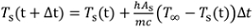 (3)
(3)
 = (Ts,j+1-Ts,j)/(tj+1-tj) (values will be negative). Here, tj is the time of each logged reading. It may be helpful to smooth these cooling rate curves by performing a running average with a sample window of 2-3 readings.
 (3)
(3)Quenching is a heat treatment commonly used to modify material properties such as hardness and ductility. During quenching and the complementary process of annealing, a material is heated and subsequently cooled. For quenching, the material is cooled very quickly in contrast to annealing where it is cooled gradually in a controlled fashion. The rate of heat transfer is determined by many factors including the thermal conductivity of an object and surrounding fluid, geometry and temperature distribution. Understanding the interplay between these factors is important for building the link between a particular heat treatment and the resulting change in material properties. This video will focus on quenching and show how to perform a simple analysis of the heat transfer during this process.
After a sample is heated, quenching requires rapid heat transfer to the surrounding environment which is commonly achieved by immersing the sample in a fluid bath such as water or oil. Heat transfer to the surrounding fluid can be driven by free convection, where local heating by the sample results in buoyancy driven circulation or forced convection, where the sample is moved through the fluid. At higher sample temperatures, bubble formation can increase the heat transfer rate, an effect known as boiling enhancement. However, if the sample becomes blanketed by low thermal conductivity vapor, there is a boiling crisis and the heat transfer will be reduced. In general, the sample temperature is not well defined because the temperature distribution inside the sample is not uniform as it cools. In other words, the temperature doesn't just depend on time, it depends on the position within the sample as well. However, if the internal heat transfer resistance is small relative to the external thermal resistance from the surface to the surrounding fluid, the sample temperature can be assumed to remain nearly uniform throughout and the analysis is simplified. The balance between these two resistances is expressed quantitatively by the Biot number, a dimensionless quantity named after the 19th century French physicist, Jean-Baptiste Biot. The Biot number is the ratio of the internal heat conduction resistance to the external convection resistance. The internal conduction resistance is the characteristic length scale of the object divided by its thermal conductivity. The external convection resistance is one over the convection coefficient. Generally, when the Biot number is less than 0.1, the temperature distribution inside the sample will remain nearly uniform. In this regime, a lumped capacitance analysis can be used to model the heat transfer rate by balancing the internal energy loss of the sample with the convective heat removal rate from Newton's Laws of Cooling. The result is a first order differential equation for the sample temperature. In the next section, we will demonstrate these principles by quenching a small, solid, copper cylinder which is representative of small, heat-treated parts.
The test piece will be made from a length of 9.53 mm copper rod. Before proceeding, calculate the Biot number to justify the use of a lumped capacitance analysis. Assume that the external conduction coefficient will not exceed 5,000 watts per meter squared Kelvin and use the characteristic length for a cylinder which is half the diameter. Look up a published value for the thermal conductivity of copper and calculate the result. Since the Biot number is less than 0.1, proceed with the preparation of the test piece. Take a section of stock and cut approximately 25 mm from the end. Remove any rough edges on the piece and then measure the mass and final length. Near each end, drill a thermal cupel well, 1.6 mm in diameter, down to the central axis. The well should be deep enough to embed the entire thermal cupel tip. These wells are relatively small so they will not have a significant effect on the overall heat transfer behavior. Next, use high-temperature epoxy to seal a high-temperature thermal cupel probe into each well. Ensure that the probe tips are completely encased and pressed into the center of the test piece as the epoxy sets. Otherwise, the probes may measure the water-bath temperature instead of the sample temperature. Once the test piece is prepared, set up the quenching bath. Insert a reference thermal cupel into the bath near where the sample will be quenched. Connect all three thermal cupels to a data acquisition system. Set up a program to continuously log transient temperature measurements around ten times per second. Everything is now prepared to perform the experiment.
This experiment requires open-flame heating so before you begin ensure that a fire extinguisher is on hand and that no flammable materials are nearby. Follow all standard precautions for fire safety. Set up the burner near the quenching bath and light the flame. Pick up the test piece by the thermal cupel leads and from a safe holding distance, gradually heat it over the flame until it reaches the desired temperature. Now start the data acquisition and immerse the test piece into the quenching bath. Hold the piece as steady as possible to minimize heat transfer by forced convection. While the sample is cooling, watch for and note any boiling behavior. When the sample temperature drops to within a few degrees of the bath temperature, stop the data acquisition program. Repeat this procedure for progressively higher initial sample temperatures up to around 300 degrees Celsius.
Open one of the data files. At every time step, there is one reading of the bath temperature and two of the sample temperature. Perform the following calculations for each time. Compute the average sample temperature by taking the arithmetic mean of the two sample readings. Calculate the instantaneous cooling rate which is the change in temperature divided by the change in time between two successive measurements. Then smooth the results with a two-point moving average to filter out some of the measurement noise. Use the differential equation derived from the lumped capacitance analysis to calculate the instantaneous heat transfer coefficient. The heat transfer coefficient can also be predicted using theoretical or empirical derived heat transfer models. These models generally report the convection coefficient in terms of the Nusselt number, a non-dimensional quantity. Consult the text for details on how to perform this calculation. With the equations for the theoretical heat transfer coefficient, you can also predict the sample cooling over time. To do this, take a starting point from your experimental data where the sample temperature is below 100 degrees Celsius. Choose a small numerical time step and assume that the bath temperature remains constant. Now, numerically integrate the differential equation from the lumped capacitance analysis. Soon, we will compare this theoretical prediction with our measurements. After you repeat this analysis for every data file, you are ready to look at the results. Plot the sample temperature versus time for a single test along with the theoretical prediction. The faster initial cooling rate is likely due to the forced convection as the sample is dropped into the bath. And later oscillations might be caused by small motions from the person holding the sample. Since the temperature prediction is soon set only free convection occurs, it is better to initialize the integration from a point after the forced convection stops. When this step is taken, the theory very accurately predicts how the sample cools over time. Now, plot the heat transfer coefficient against the sample to bath temperature difference for all of the tests together. Add the theoretical prediction for the heat transfer coefficient below the boiling point. Note the sharp rise at higher sample temperatures as the boiling process becomes more vigorous. In this experiment only boiling enhancement is observed. The low bulk fluid temperature in this case, prevents the onset of a boiling crisis.
Now that you are more familiar with the quenching process, let's look at some ways in which it is applied in the real world. Heat treatment such as quenching and annealing are critical steps in the manufacture of durable tooling. Certain steel alloys can be annealed to reduce hardness for machining and working. Once formed, they can then be quenched to achieve high hardness. Many engineered components, such as computer processors, experience large temperature fluctuation throughout their life cycle. Processors heat up rapidly when running computationally intensive programs and the temperature rise triggers increased fan speeds to enhance cooling. The prediction and characterization of heat transfer rates is important for designing components that won't fail due to overheating or fatigue.
You've just watched Jove's Introduction to Quenching. You should now understand how this common heat treatment is performed as well as some of the major factors that effect heat transfer during the quenching process. You should also know how to perform a lump capacitance analysis to predict the change in temperature and how to use the Biot number to determine when this analysis is justified. Thanks for watching.
Subscription Required. Please recommend JoVE to your librarian.
Results
Photographs of boiling at different initial sample temperatures (Ts,0) are presented in Fig. 2. At Ts,0 = 150°C vapor bubbles form and stay attached to the sample. At Ts,0 = 175°C bubbles detach and float into the water. At 200°C, more bubbles are generated, and further increases are observed at higher temperatures. Boiling crisis type events (e.g., whole sample being surrounded by persistent vapor) are not observed due to the low bulk fluid temperature (~22°C).
When the sample temperature is below the boiling temperature of the coolant (100°C), single-phase free convection models can be applied to predict the convection coefficient. The free convection heat transfer rate depends on the fluid Prandtl number (Pr), which is the ratio of viscosity to thermal diffusivity (Pr = 6.6 for water at room temperature) and the Rayleigh number (Ra), which is a measure of natural convection transport:
 (4)
(4)
Here, g is the gravitational acceleration (9.81 m s-2), β is the thermal expansion coefficient of the fluid (relative change in density with temperature, 2.28 × 10⁻⁴ K-1 for water), and ν is the fluid kinematic viscosity (9.57 × 10⁻⁷ m2 s-1 for water). As an example, for the 9.5 mm diameter sample at Ts = 75°C in water at T∞ = 22°C, the Rayleigh number is Ra = 7.44 × 10⁵.
For a horizontal cylinder in single-phase free convection heat transfer, a widely used convection formula (based on curve fits to empirical data) is presented in Equation 4.
 (5)
(5)
Here, k is the fluid thermal conductivity (0.60 W m-1 K-1 for water). The formula gives the Nusselt number (Nu), the dimensionless convection heat transfer coefficient. It can be converted to the dimensional heat transfer coefficient (h in units W m-2 K-1) by multiplying by k/D. For the example case with Ra = 7.44 × 10⁵, this model predicts Nu = 16.4 and h = 1040 W m-2 K-1.
In Fig. 3, measured instantaneous convection coefficients are compared with theoretical free convection values from Equation 4. Qualitatively close agreement is observed at lower surface temperatures (Ts-T∞ < 80 K). At higher sample temperatures, boiling occurs and measured heat transfer coefficient values significantly exceed the single-phase free convection predictions. The convection coefficient increases sharply with sample temperature at boiling conditions. This increase is due to the greater number of active nucleation sites at higher surface temperatures.
In Fig. 4, measured and predicted sample cooling curves are presented for a case with initial temperature 42.5°C. Initially, the experimental temperature curve decays quicker. This may be due to forced convection effects from inserting the sample into the bath. Over time, slight oscillations in the measured curve are observed, possibly due to motion of the person holding the sample. Later, the experimental and predicted temperature curves match well.

Figure 2: Photographs of boiling phenomena on quenched sample at increased initial temperature (T0)

Figure 3: Comparison of measured free convection and boiling convection coefficients with theoretical free convection values

Figure 4: Comparison of measured and predicted cooling curve for case with initial temperature T0 = 42.5°C
Subscription Required. Please recommend JoVE to your librarian.
Applications and Summary
This experiment demonstrated the process of transient heat transfer during quenching. The temperature of a material sample was tracked as it was rapidly cooled in a water bath. The convection coefficients and temperature profiles over time were compared with theoretical values for free convection cooling. Boiling phenomena were also discussed and observed for high initial sample temperatures. Information from such experiments and demonstrated modeling approaches can be applied to understand and design heat transfer processes for manufacturing and material heat treating.
Rapid quenching cooling is often employed in heat-treating tools. Certain steel alloys can be annealed (heated and gradually cooled) to reduce hardness for machining and working. They can then be heated and rapidly cooled to achieve high hardness for cutting other materials (e.g., files, saw blades) or in high wear applications (e.g., hammer heads, punches). Additional heat treating operations can improve toughness to prevent brittle failure.
More generally, fast transient heating and cooling is found in many applications. For example, computer processors heat up rapidly when running computationally intensive programs. This temperature rise often triggers increased fan speeds and rapid cooling. When power plants are brought online, steam generator tubes experience rapid heating. In both cases, prediction and characterization of heating and cooling rates are important to prevent materials from failing due to overheating and fatigue. Transient heat transfer analyses, as demonstrated in this investigation, are critical for engineering such technologies.
Subscription Required. Please recommend JoVE to your librarian.