Advanced Animal Model of Colorectal Metastasis in Liver: Imaging Techniques and Properties of Metastatic Clones

Summary

The ability of metastatic clones to colonize distant sites depends on their proliferation capacity and/or their ability to survive in the host microenvironment without significant proliferation. Here, we present an animal model that allows quantitative visualization of both types of liver colonization by metastatic clones.

Abstract

Patients with a limited number of hepatic metastases and slow rates of progression can be successfully treated with local treatment approaches^1,2. However, little is known about the heterogeneity of liver metastases, and animal models capable of evaluating the development of individual metastatic colonies are needed. Here, we present an advanced model of hepatic metastases that provides the ability to quantitatively visualize the development of individual tumor clones in the liver and estimate their growth kinetics and colonization efficiency. We generated a panel of monoclonal derivatives of HCT116 human colorectal cancer cells stably labeled with luciferase and tdTomato and possessing different growth properties. With a splenic injection followed by a splenectomy, the majority of these clones are able to generate hepatic metastases, but with different frequencies of colonization and varying growth rates. Using the In Vivo Imaging System (IVIS), it is possible to visualize and quantify metastasis development with in vivo luminescent and ex vivo fluorescent imaging. In addition, Diffuse Luminescent Imaging Tomography (DLIT) provides a 3D distribution of liver metastases in vivo. Ex vivo fluorescent imaging of harvested livers provides quantitative measurements of individual hepatic metastatic colonies, allowing for the evaluation of the frequency of liver colonization and the growth kinetics of metastases. Since the model is similar to clinically observed liver metastases, it can serve as a modality for detecting genes associated with liver metastasis and for testing potential ablative or adjuvant treatments for liver metastatic disease.

Introduction

Patients with liver metastases from primary colorectal cancers (CRC) are characterized by a poor prognosis. The 5-year survival rate for primary nonmetastatic CRC (stages I - III) is estimated as 75 - 88%^3,4, while patients with liver metastases (stage IV) have a 5-year survival rate of only 8 - 12%^5,6. However, metastatic patients represent a heterogeneous group, presenting with different numbers of metastases and different recurrence times. Clinical observations indicate that the number of metastases (which may be proportional to colonizing ability or frequency of colonization) and the size of any single metastasis (proportional to the local growth rate) are independent prognostic factors^1,7. In other words, the success of metastatic clones colonizing the liver depends on two major properties: their ability to grow and their ability to disseminate and survive in the liver microenvironment.

The design of successful clinical models with the capability of capturing and quantifying the properties of metastatic clones can drastically improve our understanding of liver metastasis biology and provide an effective tool for the design of potential therapeutic approaches. Models of experimental liver metastasis have been previously reported^8,9, but neither of them provided the ability to quantitatively capture and describe properties of individual metastatic clones both in vivo and ex vivo.

Here, we present a new, advanced model of liver metastasis that includes the generation of tumor clones with different liver colonization efficiencies and growth properties. We employed a combination of dual-labeling of cancer cells with luciferase and tdTomato fluorescent protein with the generation of monoclonal cell lines that have intrinsic differences in metastatic capacity. In this experimental model, the data indicate that the development of liver metastases can be described in terms of colonization frequency and doubling time (Td), which is consistent with clinical observations. The quantitative nature of this model makes it easily adoptable for drug discovery and diagnostic purposes.

Protocol

All animal procedures were approved by the Institutional Animal Care and Use Committee at the University of Chicago (Protocol # 72213-09) and performed under sterile conditions.

1. Preparations

1. Make 500 mL of medium for the culture of HCT116 tumor cells: Dulbecco's Modified Eagle Medium (DMEM) supplemented with 10% Fetal Bovine Serum (FBS), 100 U/mL penicillin, and 100 mg/mL streptomycin.
2. Autoclave the instruments to be used for the spleen injection model, including 3 - 4 surgical towels, gauze, two small Adson pickups, a needle driver, two pairs of scissors, a small clamp, and 3 microclips, at 251 °F for 20 min.
3. Prepare postoperative anesthesia for the mice, to be administered subcutaneously following the spleen injection. Dilute 2 - 4 µg of buprenorphine in 500 µL of 0.9 normal saline per mouse.
4. Prepare aliquots of 150 µg/150 µL of firefly luciferin for intraperitoneal injections during the bioluminescence assays. Store at -20 °C and protect from light.

2. Generation of Luciferase/tdTomato-labeled Monoclonal Cell Lines ^10,11

1. Thaw and maintain HCT116 human colorectal cancer cells and 293FT human embryonic kidney cells in DMEM with 10% FBS, 100 U/mL penicillin, and 100 mg/mL streptomycin. Maintain in culture at 5% CO₂ and 37 °C.
2. Produce a high-titer lentivirus.
   1. On D 1, plate 10 - 12 x 10⁶ 293FT cells between passage 3 and 10 in 15 cm cell culture dishes in 18 mL of complete DMEM (cDMEM) with 10% FBS, 1% penicillin/streptomycin, and 1% nonessential amino acids. Incubate at 37 °C and 5% CO₂.
   2. On D 2, transfect the cells using the following transfection solution:
      1. For each dish, use the following: a DNA mixture of 37.5 µg of pFUG lentiviral vector inserted with the luciferase (Luc2) and tdTomato constructs¹¹ (a gift from Dr. Geoffrey Greene at the University of Chicago), 25 µg of pCMVΔ8.74, and 12.5 µg of pMD2.G resuspended in a total of 1,062 µL of sterile H₂O. Add 188 µL of 2 M CaCl₂.
      2. Add 1,250 µL of 2x Hepes-buffered Saline (HBS, 50 mM Hepes, 1.5 mM Na₂HPO₄, and 180 mM NaCl, pH 7.12) to the DNA/CaCl₂ solution, a drop at a time, while blowing bubbles through the solution with a pipette.
      3. Incubate at RT for 20 min, and then add 15.5 mL of RT cDMEM and chloroquine to make a final concentration of 25 µM.
   3. Aspirate the media in each dish of 293FT cells and replace with the transfection solution. Add 16 mL of the transfection solution slowly, as the plated cells easily dislodge.
   4. On D 3, after 8 - 16 h, remove the transfection solution and wash the cells once with Dulbecco's Phosphate-buffered Saline (DPBS), again taking care not to dislodge the cells. Replace the media with 18 mL of fresh cDMEM with 10 mM Hepes.
      NOTE: Slowly move dishes, aspirate the transfection solution, and add the media through the sidewall of plates so as not to dislodge the cells.
   5. On D 4, at 48 h from the time of transfection, collect the media from the dishes by aspirating slowly with a pipette so as not to dislodge the cells. Centrifuge the collected media at 300 x g for 5 min to precipitate the large cell debris.
   6. Filter the viral supernatant using a 0.45 µm low-protein-binding filter flask and centrifuge using a SW-28 rotor for 2 h at 50,000 x g and 4 °C. Decant the supernatant immediately after the centrifugation finishes and dry the inside of the tube with wipers.
   7. Resuspend the viral pellet in 50 µL of Reduced Serum Medium (RSM) with 1% FBS. Aliquots can be stored at -80 °C for future use (viral stock).
3. Transduce the lentiviruses into the HCT116 cells and generate a panel of tdTomato-positive clones.
   1. Plate the HCT116 cells at a density of 1 x 10⁵ in 24 well plates 1 d before the viral infection.
   2. Dilute 40 µL of resuspended virus (from 2.2.7) in 4 mL of RSM (1:100 dilution) with 1% penicillin/streptomycin and 8 µg/mL polybrene (cRSM).
   3. On the day of infection, wash the cells once with DPBS, and then add 250 µL of diluted virus from step 2.3.2 to each well. Incubate for 4 h at 37 °C and 5% CO₂, and then add 1 mL of cDMEM to each well; incubate at 37 °C and 5% CO₂ for 48 - 72 h.
   4. Resuspend the cells with 1 mL of 0.05% trypsin and 0.53 mM EDTA, and then add 1 mL of cDMEM to neutralize the trypsin. Transfer the cells to a microcentrifuge tube and pellet at 300 x g for 4 min. Wash the pellet 3x in 1 mL of Hanks' Balanced Salt Solution (HBSS) plus 2% FBS.
   5. Resuspend the pellet from step 2.3.4 with FACS buffer (2% FBCS and 2 mM EDTA in PBS) into a single-cell suspension at 1 x 10⁶ cells/mL.
   6. Sort the tdTomato-positive HCT116 cells using a cell sorter, gating for PE-positive cells (excitation/emission: 556/585 nm). Grow the collected cells in a 10-cm dish at 5% CO₂ and 37 °C to generate parental tdTomato-positive HCT116 cells (Figure 1A).
   7. Resuspend the parental tdTomato-positive HCT116 cells from 2.3.6 with 8 mL of 0.05% trypsin and 0.53 mM EDTA for 3 - 5 min, and then add 8 mL of cDMEM to neutralize the trypsin.
      1. Transfer the cells to a 50 mL tube and pellet at 300 x g for 4 min. Remove the supernatant and dilute the parental tdTomato-positive HCT116 cells to 1 cell per 200 µL in cDMEM (Figure 1B).
   8. Plate a single cell (200 µL of the dilution) per well in a 96-well plate at 5% CO₂ and 37 °C (Figure 1C).
   9. Grow individual monoclones in flasks at 5% CO₂ and 37 °C. (Figure 1D).

3. Calibration of Fluorescent Signal Intensity as a Function of Cell Number

1. Plate the transfected HCT116 cells, now referred to as HCT116-L2T, at a density of 0, 10³, 2 x 10⁴, 3 x 10⁵, 5 x 10⁴, 7 x 10⁴, 9 x 10⁴, and 10⁵ cells/well in 96 well plates in triplicates for each density.
2. After 5 h of incubation, quantify the tdTomato fluorescent intensities using IVIS¹⁰.
   1. Click on the image software icon on the desktop to start the software. Click the "Initialize" button to initialize the imaging system. After initialization finishes (which takes about few min), select "Fluorescence", "4 second" exposure time, "Medium" binning, "2" F/stop, "535" excitation filter, and "580" emission filter.
   2. Place the 96 well plate on the imaging station and click on "Acquire" to start imaging. After the image is acquired, click "ROI Tools" in the tool palette and select 12 x 8 from the slit icon.
   3. Create 12 x 8 slits to cover the area of signal on the image of the 96 well plate and click the measurements tab. Observe a window with a table of ROI measurements with units of photons per s per steradian per square cm (photons/s/sr/cm²).
3. Construct a scatterplot with the argument (X axis) equal to the number of cells and the function (Y axis) representing signal intensity. Calculate regression curves using a data analysis software to calculate the amount of cells corresponding to the unit of fluorescent intensity (Figure 2)¹⁰.

4. Animal Model of Liver Metastases

1. Once the HCT116-L2T cells reach 70 - 80% confluency, prepare them approximately 1 h prior to the spleen injection. Dissociate the cells using 0.05% Trypsin in 0.53 mM EDTA for 3 - 5 min, and then neutralize them with an equal amount of cDMEM. Make sure to pipette thoroughly to avoid clumping.
2. Count the cells with an automatic cell counter.
3. Resuspend the cells in 1x DPBS to a concentration of 1.2 - 2 x 10⁶ cells/100 µL. Make sure to pipette and resuspend the cells thoroughly to avoid clumping.
4. Keep the cells on ice until injection, occasionally resuspending them in the tube.
5. Prior to anesthetizing the mice, provide a preoperative anesthetic and fluid bolus by subcutaneously injecting 500 µL of the buprenorphine mixture described in step 1.3. Administer the same dose of additional buprenorphine mixture twice a day until signs of pain(reduced mobility, hunched stature, failure to groom, vocalization when handled) have resolved.
6. Anesthetize 6- to 8-week-old female athymic nude mice with 2% isoflurane in oxygen in an anesthesia chamber. Confirm that the mice are completely under anesthesia by pinching the tail. Use vet ointment on the eyes to prevent dryness while under anesthesia. Transfer each anesthetized mouse to an individual nose cone for the spleen injection. Prior to incision, each mouse should be covered with a sterile surgical drape.
7. Identify the spleen as a purple area seen externally through the skin on the left flank of the nude mice. Using microdissection scissors, make an 8 mm left flank incision on the skin just above the spleen.
   1. Next, lift up on the abdominal wall and make a small incision. Allow air into the abdominal cavity so that the internal organs move away from the incision site. Enlarge the abdominal wall incision to approximately 5 mm.
   2. Expose the spleen by gently applying pressure around the incision with a cotton swab. If needed, the pancreatic fat can be gently manipulated to help with exposure so as not to injure the spleen.
8. Slowly inject 100 µL of cells using a 1 mL syringe with a 27 G needle into the tip of the exposed spleen. Inject slowly, over a period of at least 30 - 60 s, to avoid extra-liver tumors.
9. Place a microclip on the spleen prior to removing the needle at the end of the injection to prevent leakage of the injected cell suspension.
10. Leave the microclip in place for 5 min.
11. 5 min postinjection, perform a splenectomy using a hand-held cautery device for hemostasis. Dissect the splenic hilum, starting from the anterior side. When dissecting large vessels, pre-coagulate the proximal side of the vessels with adjacent fat tissue, using cautery to avoid excessive bleeding.
    NOTE: Methods for hemostasis: coagulate the bleeding point directly with cautery, apply pressure to the bleeding point for 3 - 5 min, or suture-ligate the bleeding point with a 5-0 silk tie.
12. Close the flank incision of each mouse in two layers. First, close the abdominal wall with a 5-0 absorbable braided suture (e.g., vicryl) in a single horizontal stitch. Next, close the skin using a 4-0 nonabsorbable monofilament suture (e.g., prolene), again with a single horizontal stitch.
13. Clean all instruments by spraying 70% isopropanol to maintain sterile conditions between every procedure.
    NOTE: Make sure the animals are warmed while they awake from anesthesia. Monitor all mice post-operatively until they become ambulatory and return to normal activity. Typically, the recovery time is approximately 3 - 5 min. Do not leave animals unattended until they have regained sufficient consciousness to maintain sternal recumbency. Do not return an animal that has undergone surgery to the company of other animals until it has fully recovered.

5. In Vivo Bioluminescent Imaging

1. Perform imaging on a weekly basis to measure and quantify changes in bioluminescence over time.
2. Place mice in an anesthesia chamber and anesthetize them with 2% isoflurane in oxygen. Confirm that the mice are completely under anesthesia by pinching the tails. Use vet ointment on the eyes to prevent dryness while under anesthesia.
3. Next, intraperitoneally inject each mouse with 150 µL of the preprepared firefly luciferin from step 1.4.
4. Place the mice in an IVIS with individual nose cones administering isoflurane. Place the mice in the supine position with spacers in between to minimize the signal to adjacent mice. A maximum of five mice may be imaged at one time.
5. Measure and analyze bioluminescent intensities 3 min after luciferin injection.
   1. After initializing the IVIS as described in step 3.2.1, select "Luminescent", "1 second" exposure time, and "Medium" binning.
   2. Click the "Acquire" button to start imaging. Make sure to perform each imaging at a consistent time (3 min) after the luciferin injection.
   3. After the image is acquired, an image window and tool palette will appear. Click "ROI Tools" and select "1", "2", "3", "4", or "5" from the circle icon, corresponding to the number of mice imaged.
   4. To define Regions of Interest (ROIs), circle the signal area of the luminescent signal in the abdominal cavity of the mouse, and then click "measurements" of the ROI as an arbitrary unit of radiant efficiency ((photons/s/cm²/steradian)/(µW/cm²)). Make sure to have an additional ROI circle of the background.
6. At four weeks post-injection and prior to animal sacrifice, perform Diffuse Luminescent Imaging Tomography (DLIT) using IVIS to evaluate the tumor burden and distribution using real-time 3D reconstruction of bioluminescent intensities of individual tumor colonies.
   1. Anesthetize the mice and inject luciferin, as described in step 5.2.4. DLIT is performed on one mouse at a time.
   2. After initializing the IVIS, as described in step 3.2.1, select "Imaging wizard", "Bioluminescence", and click "Next". Select "DLIT" and click "Next". Select "Firefly" probes and click "Next". Select "mouse" image subject, "Auto" exposure parameter, "C-13 cm" field of view, and "0.5 cm" subject height, and click "Next". Click the "Acquire" button to start imaging.
   3. After the image is acquired, select the "DLIT 3D Reconstruction" tab and the "Analyze" tab and click "Reconstruct" to generate the 3D reconstruction image.
   4. Click "Tools" and "3D Animation". Select "Spin CCW on Y-axis" in the 3D animation window. Click "Record" and "Save" into a .mov format file.

6. Ex Vivo Fluorescent Imaging

1. Sacrifice the mice by cervical dislocation while anesthetized, or according to institutional guidelines at 4 - 6 weeks following the spleen injections.
2. Harvest the liver. Make a horizontal incision from the left to right flank. Grabbing the xiphoid process with a pickup, dissect the falciform, the hepatic vein, and the inferior vena cava.
   1. Dissect the right hepatorenal ligament, the hepatoduodenal ligament, and the left hepatorenal ligament, taking care not to injure the caudate lobe while dissecting the hepatoduodenal ligament. After harvesting the liver, remove the gallbladder, as this will display autofluorescence. Make note of any additional extra-liver tumors present.
3. Take note of the numbers and sizes of liver tumors present macroscopically, and place the harvested livers in DPBS.
   NOTE: Tumors are macroscopically visible to the naked eye as white tumors (for a representative example, see Figure 4).
4. Prior to placement on the imaging sheet, take each liver and gently remove excess liquid by blotting on a paper towel.
5. Measure the fluorescent intensities from each tumor colony using the IVIS.
   1. Select "Fluorescence", "4 seconds" exposure time, "Medium" binning, "2" F/stop, "535" excitation filter, and "580" emission filter. Click the "Acquire" button to start imaging.
   2. After acquiring the image, locate the image window and tool palette. Click "ROI Tools" and select "1" from the circle icon. To define ROIs, circle the signal area of individual tumor colonies on the image, and then click "measurements" of the ROI as an arbitrary unit of radiant efficiency ((photons/s/cm²/steradian)/(µW/cm²)). Make sure to have an additional ROI circle of the background.
6. Calculate the total tumor volume by assuming it to be a sphere. Tumor volume = 4 x π x r³ / 3 (r = radius). Calculate the fraction of tumor colony forming cells (Fc) as the number of tumors in the liver divided by the number of cells splenically injected.
7. Calculate the total cell number per colony (=X) from the linear approximation from step 3.3. Calculate the number of cell divisions (=Y) as Y = log₂X and the Td as Td (day) = 28 / Y.

Representative Results

The goal of this experiment was to establish a consistent and easily reproducible animal model with the potential for the serial quantification of the in vivo metastatic tumor burden and for the estimation of the colonizing frequency and growth kinetics of developing liver metastases. Figures 2-6, with legends, are provided from our previous publication under a Creative Commons CC-BY license¹⁰.

Generation of Double-labeled Tumor Cell Monoclones

First, a panel of luminescent and fluorescently labeled monoclonal cell lines was generated with different metastatic abilities. Following successful transfection of luminescent (Luc2) and fluorescent (tdTomato) proteins in parental HCT116 colorectal cancer cells, 16 double-labeled monoclones were generated by diluting the parental HCT116-L2T cells to 1 cell/200 µL in 96 well plates (Figure 1)¹⁰. In vitro fluorescence and luminescence of HCT116-L2T was then quantified using an increasing amount of cells to estimate the number of tumor cells from in vivo and ex vivo liver tumor imaging (Figure 2)¹⁰.

Metastases Development by Clones with Differential Liver Colonization

Next, to generate liver metastases, the 16 previously generated individual HCT116-L2T clones were intrasplenically injected into mice; a splenectomy was then performed. The development of liver metastases was monitored by weekly in vivo bioluminescent imaging, followed by ex vivo fluorescent imaging after sacrificing the mice. Out of the 16 monoclones generated, we selected clones designated as P1, P2, O1, and O2, due to their different observed colonization and growth capabilities in the liver. Clones O1 and O2 had a smaller tumor burden, representing "oligometastatic" clones, and potentially recapitulating a phenotype of limited metastatic disease. Clones P1 and P2 had a larger tumor burden, representing widespread dissemination, which is also referred to as polymetastatic disease. The bioluminescence was higher in the P1 and P2 mice (6.7×10⁶ ± 4.7×10⁶ and 3.6×10⁶ ± 2.5×10⁶ photons/s/cm²/steradian) as compared with the O1 and O2 mice (2.0×10⁵ ± 1.3×10⁵ and 1.7×10⁵ ± 9.1×10⁴ photons/s/cm²/steradian) 3 weeks after the spleen injection (Figure 3A, B)¹⁰. The quantification of ex vivo fluorescence of the livers at 4 weeks after the spleen injection demonstrated that P1 and P2 livers had higher fluorescent intensities compared with O1 and O2 livers (Figure 3C). The tumor distributions in the ex vivo fluorescent images were consistent with macroscopic findings (Figure 3C, D)¹⁰.

Colonization and Growth Kinetics of Individual Clones

The numbers and sizes of tumors visualized macroscopically were counted and measured in each individual liver. In addition, ex vivo fluorescence imaging was done on each individual tumor colony for each monoclone (Figure 4)¹⁰. The total number of tumors in P1 was higher, as compared to P2, O1, and O2, while the size of tumors was larger in P2 than in P1, O1, and O2 (p <0.001; Figure 5A, B)¹⁰. However, the total tumor volume in the liver in P1 and P2 was larger as compared to O1 and O2 (Figure 5C)¹⁰. The Fc, which indicates the ability of tumor cells to colonize the liver, is calculated as the number of tumors in the liver divided by the number of cells injected. Using this method, there is an assumption that the number of tumors in the liver corresponds to the number of cells that have an ability to colonize the liver. Thus, P1 had an enhanced ability to colonize the liver when compared to the other clones (Fc = 8.2×10⁻⁵ ± 1.1×10⁻⁵, 6.0×10⁻⁶ ± 2.3×10⁻⁶ in P1 and O1, respectively, p <0.001; Figure 5D)¹⁰. Though P2 had a similar ability to colonize the liver as clones O1 and O2, the size of the tumors generated was larger than the other clones. The total number of cells per tumor colony, the Td, and the number of cell divisions can be calculated from this data by using the calibration previously generated from the correlation between fluorescent intensity and the number of cells (Figures 2 and 5E - G)¹⁰. P1, which generated many small tumors in the liver, as seen by macroscopic visual inspection, had a larger Fc, though it had a Td similar to O1 and O2 (p <0.05). P2, which generated a limited number of macroscopic large tumors, had a similar Fc but a shorter Td compared to O1 and O2 (p <0.05). Taken together, these results indicate that the Fc and Td are two key parameters contributing to metastatic potential.

The 3D distribution of metastatic tumors in the liver was demonstrated by DLIT (Figure 6)¹⁰. Using this imaging technique, it is possible to monitor spatial-temporal dynamic behavior of the metastases by the detection and measurement of the bioluminescence of individual hepatic metastatic colonies.

Statistical Analysis

The data generated was analyzed using standard data analysis software, and error bars were demonstrated as the mean ± standard deviation. Pearson's correlation coefficients were used to evaluate associations between parameters. P values were assessed using 2-tailed Student's t-tests, with a p < 0.05 considered to be statistically significant.

Figure 1: Generation of a Panel of Monoclones of Labeled HCT116 Cells. (A) Grow parental HCT116 cells labeled with luciferase and tdTomato. (B) Dilute parental HCT116 cells to 1 cell/200 µL. (C) Plate 200 µL of the dilution in a 96 well plate. (D) Grow monoclones from each well in the 96 well plate. (E) Inject monoclones intrasplenically into mice to generate liver metastases. Please click here to view a larger version of this figure.

Figure 2: Estimation of the Number of Cells by Fluorescent Intensities. (A) The luminescent image of different numbers of cells triplicated in a 96 well plate. (B) The correlation between the number of cells and the luminescence (R = 0.99, p < 0.0001). The scale bar represents luminescent intensity (photons/s/cm²/steradian). (C) The fluorescent image of different numbers of cells triplicated in a 96 well plate. Intensities were acquired as radiant efficiencies with a 535 nm excitation and a 580 nm emission. (D) The correlation between the number of cells and the fluorescence (R = 0.99, p < 0.0001). The scale bar represents the fluorescent intensity in an arbitrary unit of radiant efficiency ((photons/s/cm²/steradian)/(µW/cm²)). Reprinted with permission¹⁰. Please click here to view a larger version of this figure.

Figure 3: Bioluminescence and Ex Vivo Fluorescence of the Liver in Selected Clones. (A) Representative bioluminescent images. The scale bar represents luminescent intensity (photons/s/cm²/steradian). (B) Bioluminescence measured weekly from 1 - 3 weeks in P1 and P2, and 1 - 4 weeks in O1 and O2. Data were represented as the mean ±standard deviation. (C) Representative ex vivo fluorescent images of livers. Intensities were acquired as radiant efficiencies with a 535 nm excitation and a 580 nm emission. The scale bar represents fluorescent intensity in an arbitrary unit of radiant efficiency ((photons/s/cm²/steradian)/(µW/cm²)). (D) Macroscopic liver images (arrows indicate small white tumors). P1 and P2: polymetastatic clones, O1 and O2: oligometastatic clones. Reprinted with permission¹⁰. Please click here to view a larger version of this figure.

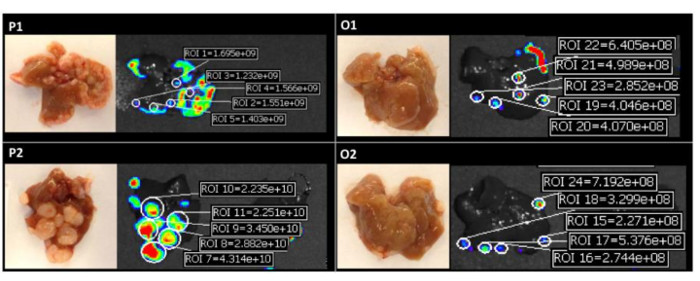
Figure 4: Quantification of Fluorescent Intensities of Individual Liver Colonies. Images on the left are representative macroscopic findings and images on the right are fluorescent intensities in each clone. The fluorescent intensities were acquired as radiant efficiencies with a 535 nm excitation and a 580 nm emission. P1 and P2: polymetastatic clones, O1 and O2: oligometastatic clones. Reprinted with permission¹⁰. Please click here to view a larger version of this figure.

Figure 5: Quantitative Estimation of Colonizing Ability and Growth Kinetics. (A) The macroscopic total number of tumors, (B) macroscopic size of individual tumors, (C) calculated total tumor volume in the liver, (D) colonizing fraction of tumor colony forming cells (Fc), (E) total cell number per colony, (F) doubling time (Td), and (G) number of cell divisions of each clone. P1 and P2: polymetastatic clones, O1 and O2: oligometastatic clones. Data were represented as the mean ±standard deviation for all figure panels in which error bars were shown. Reprinted with permission¹⁰. Please click here to view a larger version of this figure.

Figure 6: Quantification of Bioluminescence of Individual Tumor Colonies using Diffuse Luminescent Imaging Tomography (DLIT). (A) 3D overhead view. The scale bar represents fluorescent intensity in an arbitrary unit of radiant efficiency. (B) Coronal section. (C) Sagittal section. (D) Transaxial section. (E) Macroscopic image of liver. (F) Ex vivo fluorescent image of the liver. Reprinted with permission¹⁰. Please click here to view a larger version of this figure.

Discussion

The animal model presented in the current report is based on two major approaches. First, in order to ensure the ability to observe metastatic clones with different propensities to colonize and proliferate in the liver, a panel of highly heterogeneous monoclonal cell lines was established, rather than an established unfractionated cancer cell line^12,13. The monoclonal approach to metastasis development is justified by recent genomic data¹⁴ and was successfully used previously to model the metastatic process^10,15,16. Second, double-labeling of the parental cell line by luciferase and tdTomato markers was incorporated in order to provide enhanced analysis of metastatic growth both in vivo and ex vivo. The luminescent and fluorescent labeling allows for a detailed anatomical examination and potential quantification of both the amount of metastatic tumors (considered as the frequency or efficacy of liver colonization) and the size of any individual colony. The latter can easily be converted to an actual number of cells using a simple calibration procedure described in step 2 and Figures 2¹⁰ and 4¹⁰. Using this data, it is possible to estimate the Td for each metastatic node in the liver and to evaluate the growth kinetics of liver metastases for each initial monoclone injected (Figure 5)¹⁰.

Three different colorectal metastatic phenotypes were observed in this experimental system, designated as P1, P2, and O1/O2. These metastatic phenotypes differed when comparing the data of frequency of colonization and local growth rates for each metastatic clone. The first metastatic phenotype, P1, demonstrated an enhanced ability to colonize the liver but a relatively low local growth rate, corresponding to many small metastatic tumors throughout the liver. The second metastatic phenotype, P2, had a lower frequency of colonization but a significantly higher local growth rate, resulting in a relatively small number of large secondary tumors. Lastly, the third metastatic phenotype, O1 and O2, demonstrated both a low frequency of colonization and slow local growth rates. This third metastatic phenotype may be considered as a representation of clinical oligometastatic liver disease (Figures 3¹⁰ and 5¹⁰). In addition, gene expression analysis comparing these clones¹⁰ identified significant differences in expression patterns. For example, when comparing P1 with O1 and O2 clones, there were 756 differentially expressed genes, including a subset of genes involved in inflammatory responses and interferon signaling. This study, as well as others, have implicated these genes in playing key roles in tumor growth and survival^{21, 22}. In addition, when comparing P2 to O1 and O2, there were 461 differentially expressed genes, with a subset involving genes critical to cellular growth and proliferation mediated through ERK1/2 signaling.

The diversity of metastatic phenotypes produced by this experimental model is consistent with the observed clinical representations of metastatic heterogeneity. For example, it has been shown that the size of liver metastases (a parameter related to growth potential) and their numbers (a parameter related to colonization ability) are independent risk factors for distant metastasis¹. With enhanced growth potential or colonization ability, the properties observed in P1 and P2 are consistent with these data. In addition, recent observations of patients treated with Stereotactic Body Radio-therapy (SBRT) or with surgically resected lung metastases point both to the number of tumors and the rate of progression as key factors determining overall and disease-free outcomes^17,18. Thus, colonization and growth abilities seem to be among the most critical factors in determining the development of metastatic clones at distant sites^19,20. Experimental models, which are based on these properties of metastatic clones, may provide useful tools for understanding the mechanisms of metastasis development, as well as provide a means for testing new treatment modalities for the cure of liver metastatic disease.

While an orthotopic model capable of producing spontaneous metastases is ideal, there remains a paucity of easily reproducible and consistent spontaneous models. While models utilizing intracecal implantation or injections have been described, they demonstrated variable rates of uptake and metastasis formation^23-26. Other methods have utilized an ectopic implantation approach by intrasplenic or intraportal injection to generate hepatic metastases. While the overall technique of injection is the same, the model presented here provides a sensitive approach to understanding the mechanisms of metastasis development, starting from the stage of Circulating Tumor Cells (CTC). Sensitivity and reproducibility of our approach is determined by the double-labeling of the cell lines to allow for both bioluminescent and fluorescent imaging to track the dynamics of the metastatic process. Due to the ability to quantify the metastatic burden from the luminescent and fluorescent data, it is possible to systematically measure and track the growth kinetics of metastases over time. Although alternative approaches, such as ultrasound-based imaging, have been used, these modalities are much more user-dependent, with potentially increased inter-user variability²⁷. In addition, by generating a panel of monoclonal cell lines, we are able to provide reproducible and distinct metastatic phenotypes in order to better model the variability of metastatic disease seen in the clinical setting.

While mastering this experimental technique, specifically the intrasplenic injection for the in vivo mouse model (see step 4), there are a few critical steps that may require modification. Of note, performing the splenic injection is the most important portion of the model, as an inadequate injection of the spleen may result in poor results. Leakage of cells during the injection, or leakage caused by the inappropriate placement of the microclip, may result in a lower number of liver metastases and/or a significant amount of extra-liver tumors or peritoneal carcinomatoses. In addition, it is important to inject the tumor cells slowly, for at least as long as described in the protocol, in order to avoid an increase in the intrasplenic pressure, which may lead to extravasation of the cells to adjacent tissues and the growth of extra-liver tumors around the stump of the spleen dissection.

Lastly, in step 4.3, there is a range of cells given for the splenic injection (1.2 - 2 × 10⁶ cells). The purpose of this range is to account for individual operators of this technique. It may take time to calibrate an optimal number of cells to inject. If too few cells are injected, liver metastases may not develop consistently, and if too many cells are injected, portal venous occlusion may occur, leading to the early demise of the animal. It may be prudent to initially try several different concentrations of tumor cells when starting this model in order to find the optimal number.

One pitfall of the presented model is that it is based on a xenograft approach and exploits immunodeficient nude mice. One alternative method proposed is the generation of a similar panel of monoclonal derivatives of the murine colorectal cell line MC38, double-labeled with luciferase and tdTomato or EGFP proteins. These clones can then be used in syngeneic animal models in order to capture the interactions of developing liver metastases with the host immune system.

Materials

Name	Company	Catalog Number	Comments
IVIS Spectrum In Vivo Imaging System	Caliper Life Sciences	124262	In Vivo imaging system
LivingImage 4.0 Software	Caliper Life Sciences	128165	Imaging software
VAD-MGX Research Anesthetic Machine	Vetamac	VAD-MGX	Inhalation anesthesia machine
DMEM	Gibco	11965-118	Cell culture reagents
DPBS	Gibco	14190250	Cell culture reagents
Penicillin/Streptomycin, liquid (10,000 units penicillin;10,000 μg streptomycin)	Invitrogen	15140163	Cell culture reagents
HBSS	ThermoFisher	24020117	Cell culture reagents
Buprenex Injection (0.3 mg/mL)	Reckitt Benckiser Healthcare Ltd.	12496-0757-5	Buprenorphine hydrochloride
Gemini Cautery System	Braintree Scientific	GEM 5917	Hand-held cautery for splenectomy
Micro Clip; Straight; 70 Grams Pressure; 1.5 mm Clip Width; 10 mm Jaw Length	Roboz Surgical Instrument	RS-5426	Hemoclip: Hemostasis instruments after spleen injection
D-luciferin, potassium salt	Goldbio Technology	LUCK-1G	Luciferin potassium salt
Opti-MEM I Reduced Serum Medium	Gibco	31985062	Reduced Serum Medium
TC20 Automated Cell Counter	BIO-RAD	1450102	Automatic cell counter
JMP10 software	SAS Institute		Data analysis software
BD FACSAria II cell sorter	BD Biocsiences		Cell sorter

References

- Fong, Y., Fortner, J., Sun, R. L., Brennan, M. F., Blumgart, L. H. Clinical score for predicting recurrence after hepatic resection for metastatic colorectal cancer: analysis of 1001 consecutive cases. Ann. Surg. 230 (3), 309-318 (1999).
- Pawlik, T. M., et al. Effect of surgical margin status on survival and site of recurrence after hepatic resection for colorectal metastases. Ann. Surg. 241 (5), 715-722 (2005).
- Park, J. H., Watt, D. G., Roxburgh, C. S., Horgan, P. G., McMillan, D. C. Colorectal Cancer, Systemic Inflammation, and Outcome: Staging the Tumor and Staging the Host. Ann. Surg. 263 (2), 326-336 (2016).
- Veen, T., et al. Long-Term Follow-Up and Survivorship After Completing Systematic Surveillance in Stage I-III Colorectal Cancer: Who Is Still at Risk. J. Gastrointest. Cancer. 46 (3), 259-266 (2015).
- Siegel, R., et al. Cancer treatment and survivorship statistics. CA Cancer J. Clin. 62 (2), 220-241 (2012).
- O'Connell, J. B., Maggard, M. A., Ko, C. Y. Colon cancer survival rates with the new American Joint Committee on Cancer sixth edition staging. J. Natl. Cancer Inst. 96 (19), 1420-1425 (2004).
- House, M. G., et al. Survival after hepatic resection for metastatic colorectal cancer: trends in outcomes for 1,600 patients during two decades at a single institution. J. Am. Coll. Surg. 210 (5), 744-752 (2010).
- Smakman, N., Martens, A., Kranenburg, O., Borel Rinkes, I. H. Validation of bioluminescence imaging of colorectal liver metastases in the mouse. J. Surg. Res. 122 (2), 225-230 (2004).
- Rajendran, S., et al. Murine bioluminescent hepatic tumour model. J. Vis. Exp. (41), (2010).
- Oshima, G., et al. Imaging of tumor clones with differential liver colonization. Sci. Rep. 5 (10946), (2015).
- Liu, H., et al. Cancer stem cells from human breast tumors are involved in spontaneous metastases in orthotopic mouse models. Proc. Natl. Acad. Sci. U. S. A. 107 (42), 18115-18120 (2010).
- Wang, X. M., et al. Integrative analyses identify osteopontin, LAMB3 and ITGB1 as critical pro-metastatic genes for lung cancer. PLoS One. 8 (2), e55714 (2013).
- Fidler, I. J., Kripke, M. L. Metastasis results from preexisting variant cells within a malignant tumor. Science. 197 (4306), 893-895 (1977).
- Yachida, S., et al. Distant metastasis occurs late during the genetic evolution of pancreatic cancer. Nature. 467 (7319), 1114-1117 (2010).
- Khodarev, N. N., et al. STAT1 pathway mediates amplification of metastatic potential and resistance to therapy. PLoS One. 4 (6), e5821 (2009).
- Langley, R. R., Fidler, I. J. Tumor cell-organ microenvironment interactions in the pathogenesis of cancer metastasis. Endocr. Rev. 28 (3), 297-321 (2007).
- Lussier, Y. A., et al. Oligo- and polymetastatic progression in lung metastasis(es) patients is associated with specific microRNAs. PLoS One. 7 (12), e50141 (2012).
- Lussier, Y. A., et al. MicroRNA expression characterizes oligometastasis(es). PLoS One. 6 (12), e28650 (2011).
- Calon, A., et al. Dependency of colorectal cancer on a TGF-beta-driven program in stromal cells for metastasis initiation. Cancer Cell. 22 (5), 571-584 (2012).
- Vanharanta, S., Massague, J. Origins of metastatic traits. Cancer Cell. 24 (4), 410-421 (2013).
- Khodarev, N. N., Roizman, B., Weichselbaum, R. R. Molecular pathways: Interferon/Stat1 Pathway: Role in the tumor resistance to genotoxic stress and aggressive growth. Clin. Cancer Res. 18 (11), 3015-3021 (2012).
- Li, C., et al. Interferon-stimulated gene 15 (ISG15) is a trigger for tumorigenesis and metastasis of hepatocellular carcinoma. Oncotarget. 5 (18), 8429-8441 (2014).
- Cespedes, M. V., et al. Orthotopic microinjection of human colon cancer cells in nude mice induces tumor foci in all clinically relevant metastatic sites. Am. J. Pathol. 170 (3), 1077-1085 (2007).
- Tseng, W., Leong, X., Engleman, E. Orthotopic mouse model of colorectal cancer. J. Vis. Exp. (10), (2007).
- Soares, K. C., et al. A preclinical murine model of hepatic metastases. J. Vis. Exp. (27), e51677 (2014).
- Evans, J. P., et al. From mice to men: Murine models of colorectal cancer for use in translational research. Crit. Rev. Oncol. Hematol. 98, 94-105 (2016).