Near-Infrared Temperature Measurement Technique for Water Surrounding an Induction-heated Small Magnetic Sphere

Naoto Kakuta; Keisuke Nishijima; Van Cuong Han; Yuki Arakawa; Katsuya Kondo; Yukio Yamada

doi:10.3791/57407

Engineering

Near-Infrared Temperature Measurement Technique for Water Surrounding an Induction-heated Small Magnetic Sphere

Published: April 30, 2018 doi: 10.3791/57407

Naoto Kakuta¹, Keisuke Nishijima¹, Van Cuong Han¹, Yuki Arakawa¹, Katsuya Kondo², Yukio Yamada³

¹Department of Mechanical Engineering, Tokyo Metropolitan University, ²Department of Electrical and Electronic Engineering, Tottori University, ³Brain Science Inspired Life Support Research Center, The University of Electro-Communications

ERRATUM NOTICE

Important: There has been an erratum issued for this article. Read more …

Summary

A technique utilizing wavelengths of 1150 and 1412 nm to measure the temperature of water surrounding an induction-heated small magnetic sphere is presented.

Abstract

A technique to measure the temperature of water and non-turbid aqueous media surrounding an induction-heated small magnetic sphere is presented. This technique utilizes wavelengths of 1150 and 1412 nm, at which the absorption coefficient of water is dependent on temperature. Water or a non-turbid aqueous gel containing a 2.0-mm- or 0.5-mm-diameter magnetic sphere is irradiated with 1150 nm or 1412 nm incident light, as selected using a narrow bandpass filter; additionally, two-dimensional absorbance images, which are the transverse projections of the absorption coefficient, are acquired via a near-infrared camera. When the three-dimensional distributions of temperature can be assumed to be spherically symmetric, they are estimated by applying inverse Abel transforms to the absorbance profiles. The temperatures were observed to consistently change according to time and the induction heating power.

Introduction

A technique to measure temperature near a small heat source within a medium is required in many scientific research fields and applications. For example, in the research on magnetic hyperthermia, which is a cancer therapy method using electromagnetic induction of magnetic particles, or small magnetic pieces, it is critical to accurately predict the temperature distributions generated by the magnetic particles¹^,². However, although microwave³^,⁴, ultrasound⁵^,⁶^,⁷^,⁸, optoacoustic⁹, Raman¹⁰, and magnetic resonance¹¹^,¹²-based temperature measurement techniques have been researched and developed, such an inner temperature distribution cannot be accurately measured at present. Thus far, single-position temperatures or temperatures at a few positions have been measured via temperature sensors, which, in the case of induction heating, are non-magnetic optical fiber temperature sensors¹³^,¹⁴. Alternatively, the surface temperatures of media have been remotely measured via infrared radiation thermometers to estimate the inner temperatures¹⁴. However, when a medium containing a small heat source is a water layer or a non-turbid aqueous medium, we have demonstrated that a near-infrared (NIR) absorption technique is useful to measure the temperatures¹⁵^,¹⁶^,¹⁷^,¹⁸^,¹⁹. This paper presents the detailed protocol of this technique and representative results.

The NIR absorption technique is based on the principle of temperature dependence of the absorption bands of water in the NIR region. As is shown in Figure 1a, the ν₁ + ν₂+ ν₃ absorption band of water is observed in the 1100-nm to 1250-nm wavelength (λ) range and shifts to shorter wavelengths as the temperature increases¹⁹. Here, ν₁ + ν₂+ ν₃ means that this band corresponds to the combination of the three fundamental O-H vibration modes: symmetric stretching (ν₁), bending (ν₂), and antisymmetric stretching (ν₃)²⁰^,²¹. This change in the spectrum indicates that the most temperature-sensitive wavelength in the band is λ ≈ 1150 nm. Other absorption bands of water also exhibit similar behavior with respect to the temperature¹⁵^,¹⁶^,¹⁷^,¹⁸^,²⁰^,²¹. The ν₁ + ν₃ band of water observed within the range λ = 1350−1500 nm and its temperature dependence are shown in Figure 1b. In the ν₁ + ν₃ band of water, 1412 nm is the most temperature-sensitive wavelength. Thus, it is possible to obtain two-dimensional (2D) temperature images by using an NIR camera to capture 2D absorbance images at λ = 1150 or 1412 nm. As the absorption coefficient of water at λ = 1150 nm is smaller than that at λ = 1412 nm, the former wavelength is suitable for approximately 10-mm-thick aqueous media, while the latter is suitable for approximately 1-mm-thick ones. Recently, using λ = 1150 nm, we obtained the temperature distributions in a 10-mm-thick water layer containing an induction-heated 1-mm-diameter steel sphere¹⁹. Moreover, the temperature distributions in a 0.5-mm-thick water layer have been measured by using λ = 1412 nm¹⁵^,¹⁷.

An advantage to the NIR-based temperature imaging technique is that it is simple to setup and implement because it is a transmission-absorption measurement technique and needs no fluorophore, phosphor, or other thermal probe. In addition, its temperature resolution is less than 0.2 K¹⁵^,¹⁷^,¹⁹. Such a good temperature resolution cannot be achieved by other transmission techniques based on interferometry, which have often been used in heat and mass transfer studies²²^,²³^,²⁴. We note, however, that the NIR-based temperature imaging technique is not suitable in cases with considerable local temperature change, because the deflection of light caused by the large temperature gradient becomes dominant¹⁹. This matter is referred in this paper in terms of practical use.

This paper describes the experimental setup and procedure for the NIR-based temperature imaging technique for a small magnetic sphere heated via induction; additionally, it presents the results of two representative 2D absorbance images. One image is of a 2.0-mm-diameter steel sphere in a 10.0-mm-thick water layer that is captured at λ = 1150 nm. The second image is of a 0.5-mm-diameter steel sphere in a 2.0-mm-thick maltose syrup layer that is captured at λ = 1412 nm. This paper also presents the calculation method and results of the three-dimensional (3D) radial distribution of temperature by applying the inverse Abel transform (IAT) to the 2D absorbance images. The IAT is valid when a 3D temperature distribution is assumed to be spherically symmetric as in the case of a heated sphere (Figure 2)¹⁹. For the IAT calculation, a multi-Gaussian function fitting method is employed here, because the IATs of Gaussian functions can be obtained analytically²⁵^,²⁶^,²⁷^,²⁸^,²⁹ and fit well to monotonically decreasing data; this includes experiments employing thermal conduction from a single heat source.

Subscription Required. Please recommend JoVE to your librarian.

Protocol

1. Experimental Setup and Procedures

Prepare an optical rail to mount a sample and optics for NIR imaging as follows.

Sample preparation.
Note: When using water or aqueous liquid, do Step 1.1.1. When using an aqueous gel with high viscosity, do Step 1.1.2.
1. Steel sphere setting in water.
  1. Fix a 2.0-mm-diameter steel sphere to the end of a thin plastic string using a small amount of glue.
  2. Hang the steel sphere at the center of the rectangular glass cell with an optical path length of 10.0 mm, a width of 10 mm, and a height of 45 mm (Figure 3).
  3. Pour filtered water into the cell carefully so as not to produce air bubbles.
    NOTE: A steel sphere can also be fixed to the tip of a thin plastic rod with a small amount of glue¹⁹.
2. Steel sphere setting in aqueous gel.
  1. Heat an aqueous gel to reduce its viscosity such that it is low enough to be poured smoothly.
  2. Using a syringe, pour the aqueous gel into a rectangular glass cell with an optical path length of 2.0 mm, a width of 10 mm, and a height of 45 mm to half-full and leave it to cool.
  3. Place a 0.5-mm-diameter steel sphere in the center of the gel surface.
  4. Fill the cell with the aqueous gel.
    NOTE: Larger spheres (>~1 mm dia.) should not be used with a gel because they will move by gravitational and/or magnetic forces during induction heating.
3. Set the cell in a plastic holder and mount it on the optical rail (Figure 3).
Preparation of NIR imaging system.
1. Prepare a halogen lamp with a fiber light guide, and fix the end of the fiber light guide with a holder on the optical rail.
2. Place a narrow bandpass filter (NBPF) with a transmittance peak at λ = 1150 nm or λ = 1412 nm between the fiber light guide and the cell (Figure 3).
3. Interpose another bandpass filter (BPF), whose transmission wavelength range is wider than that of the NBPF, between the halogen lamp and the NBPF.
  NOTE: The BPF is needed to prevent thermal damage to the NBPF because it receives light directly.
4. Interpose an iris diaphragm(s) in the light path between the NBPF and cell holder to reduce the stray light (Figure 3).
5. Set up an NIR camera to detect the light transmitted through the cell (Figure 3). Connect the camera through a data transfer cable to a graphic board installed in a personal computer (PC) with image acquisition software.
6. Set a telecentric lens between the cell and camera (Figure 3).
  NOTE: A common camera lens can also be used. However, a telecentric lens is better in terms of the selective detection of the light parallel to the chief ray for the IAT and reduction of the influence of diffraction.
  NOTE: The NBPF and BPF should not be placed between the cell and camera because, in doing so, the water temperature would increase via direct absorption of high-intensity light from the halogen lamp.
7. Turn on the NIR camera and launch the image acquisition software.
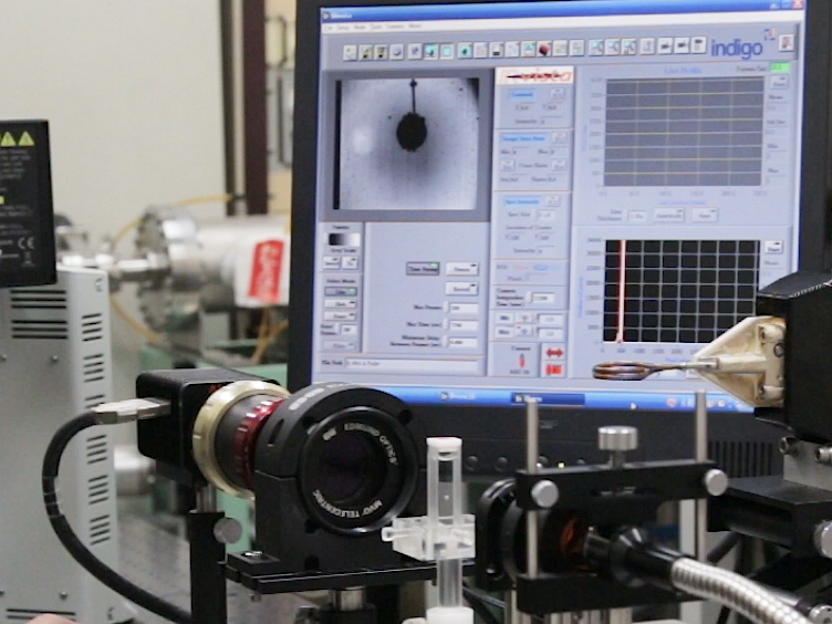
8. Light the halogen lamp and adjust its output power observing the image displayed on the monitor (Figure 4).
9. Adjust the axis, position, and focus of the telecentric lens to obtain a fine image of the steel sphere.
  NOTE: If the adjustment is not complete, irregular intensity patterns will appear, leading to incorrect absorbances.
Preparation of induction heating system.
1. Prepare an induction heating system consisting of a high-frequency generator (maximum output power: 5.6 kW; frequency: 780 kHz), water-cooled coil, and water chiller.
  NOTE: An induction heating system for brazing, welding, and soldering small metal parts is appropriate for this purpose; see Table of Materials.
2. If possible, mount the coil on an XYZ movable stage to change its position.
3. Place the coil near the cell such that the distance between the coil center and the steel sphere is approximately 15 mm (Figure 3). Ensure that there are no other metal parts near the coil.
  NOTE: The distance should be adjusted depending on the induction heating power and the sphere size.
4. Circulate water for cooling.
Image acquisition and induction heating.
1. Click "start" on the image acquisition software to store the images sequentially.
2. Click "start" on the induction heating control software to commence the induction heating.
3. After several seconds (depending on the conditions and purpose), click "stop" on the image acquisition software.
4. Click "stop" on the induction heating control software.
5. Save the temporally-stored images as a TIFF sequence (or other non-compressed format) on the image acquisition software.
  NOTE: If the temperature is high enough, the effect of light deflection will appear on the image⁷. The induction heating power must be decreased appropriately though experiments such that the increase in the temperature near the sphere is less than approximately 10 K, which can be confirmed in the following protocol steps for temperature estimation.

2. Image Processing and Temperature Estimation

Note: The saved sequential images are represented as I_i(x, z), where i is the sequential frame number. The coordinates, x, y, z, r, and r' are defined as are indicated in Figure 2; z is positive in the direction opposite to gravity. The outline of the following protocol steps is also illustrated in Supplement 1.

Absorbance image construction.
1. Open I_i(x, z) with the image processing software.
2. Reduce noise in I_i(x, z) by implementing 3 × 3 pixel averaging.
3. Create an average image of I_i(x, z) over i = 1 to 5 (or more) before heating, and define it as the reference image, I_r(x, z).
  NOTE: This averaging reduces the noise to obtain a more reliable image than a single frame image.
4. Construct the sequential images of the absorbance difference, ΔA_i(x, z), via the following equation:
  (1)
  NOTE: ΔA_i(x, z) is the variation in the absorbance, A_i(x, z), from the reference absorbance, A_r(x, z), before heating, and is derived as follows¹⁵^,¹⁶^,¹⁷^,¹⁸^,¹⁹:
  (2)
  where I₀ is the intensity of incident light to the cell.
5. Colorize the ΔA_i images using an appropriate color map such as blue-to-red.
  NOTE: The command script file for running Steps 2.1.2 through 2.1.5 for ImageJ is presented in Supplement 2.
Temperature estimation.
1. Choose the time period during which ΔA_i(x, z) is circularly symmetric with respect to the center of the sphere by visually observing the images.
  NOTE: The circular symmetry is broken mainly by free convection. An image-based analytical judgement of free convection occurring is introduced in the previous work¹⁹; however, practically, the visual judgement is effective.
2. Extract the ΔA_i(rʹ, θ) data along 360 radial lines (Δθ = 1˚) on the ΔA_i(x, z) images.
3. Exclude the ΔA_i(rʹ, θ) data within the sphere and in its vicinity (Δrʹ≈ 0.2 mm). Note: The data are anomalously very small or large in the vicinity mainly because of the slight movement of the sphere.
4. Average ΔA_i(rʹ, θ) over θ to determine the line profile, ΔA_i(rʹ).
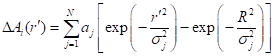
  NOTE: The command script file for running Steps 2.2.2 through 2.2.4 for ImageJ is presented in Supplement 3.
5. Approximate the ΔA_i(rʹ) data by the following multi-Gaussian function:
  (3)
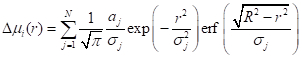
  where a_j is the weighting factor, σ_j is the dispersion parameter, and R is the maximum of rʹ where ΔA_i(R) = 0 can be assumed.
6. Calculate the absorption coefficient difference, Δµ_i(r), by substituting the obtained N, a_j, and σ_j into the following IAT of Eq. (3):
  (4)
  where erf is the error function.
7. Convert Δµ_i(r) to temperature via the following equation:
  (5)
  with the temperature coefficients of water, α_f, which are 2.8 x 10^-4 K^-1 mm^-1 for λ = 1150 nm¹⁹ and 4.1 × 10^-3 K^-1mm^-1 for λ = 1412 nm¹⁷.
  Note: The command script file for running Steps 2.2.5 through 2.2.7 is presented in Supplement 4, where the Levenberg-Marquardt nonlinear least-squares algorithm¹⁷^,¹⁹ is employed for Step 2.2.5.

Subscription Required. Please recommend JoVE to your librarian.

Representative Results

Images of ΔA_i(x, z) at λ = 1150 nm for a 2.0-mm-diameter steel sphere in water and at λ = 1412 nm for a 0.5-mm-diameter steel sphere in maltose syrup are presented in Figure 5a and Figure 6a, respectively. In both cases, the sphere was located 12 mm below the bottom of the coil along its central axis. Figure 5b and Figure 6b show the ΔA(rʹ) data and their fitted multi-Gaussian functions in Eq. (3) with R = 3.0 mm and R = 1.5 mm, respectively. No more than two or three Gaussian functions (N = 2 or 3) are needed to achieve a good fit¹⁷^,¹⁹. The fitted functions were then transformed into ΔT(r) profiles via Eqs. (4) and (5), and are presented in Figure 5c and Figure 6c.

The ΔA images in both cases clearly show an increase in the temperature of the water and gel surrounding the sphere due to thermal conduction. The circular symmetry of ΔA with respect to the sphere is observed in all images. The plots and curves in Figure 5c indicate that ΔA(rʹ) increases with time at distances nearest to the sphere; at rʹ≥ 2.5 mm, no significant change is observed. Moreover, the ΔT(r) profiles obtained via the IAT verify the occurrence of thermal conduction in the radial direction. Note that, although the ΔT(r) profiles appear similar to those of ΔA(rʹ), the changes in the dΔT(r)/dr gradient differ from those of the ΔA(rʹ) profiles. In Figure 6, the magnitudes of ΔA are found to correspond to the heating power levels, i.e., heat generation rates of the sphere.

Results for the 0.5-mm-diameter sphere demonstrate that free convection, which distorts the circular pattern in ΔA, was not observed after t = 1.2 s. Conversely, for the 2.0-mm-diameter sphere in water, free convection was found to occur after t = 1.2 s (not shown). This means that a transition from a pure thermal conduction regime to a free convection regime may have occurred in the water at approximately t = 1.2 s. This difference in free convection was caused by the differences in the heat generation rate and viscosity. The heat generation rate of the 0.5-mm-diameter sphere was significantly smaller than that of the 2.0-mm-diameter sphere; furthermore, the viscosity of the maltose syrup (approximately 100 Pa·s) was considerably higher than that of water (approximately 0.001 Pa·s). Because free convection is an important topic in heat and mass transfer research, the proposed imaging technique, which provides the onset time of free convection and pattern of the thermal plume and yields information on the physical conditions inducing free convection, will contribute significantly to research in this field.

Figure 1: Temperature dependence of NIR absorption spectrum of water. (a, b) Absorption band spectra of water at temperatures from 16.0 °C (blue) to 44.0 °C (red) in 4.0 °C increments in wavelength ranges of 1100-1250 nm and 1350-1500 nm, respectively. The arrows indicate the direction of the increase in temperature. The insets show the absorbance difference spectra; the absorbance spectra at 16.0 °C are the references. The optical path lengths are 10 mm and 1.0 mm in (a) and (b), respectively. The vertical dashed lines indicate the temperature-sensitive wavelengths of 1150 nm and 1412 nm used to obtain the NIR images. Please click here to view a larger version of this figure.

Figure 2: Coordinate system and geometry for absorbance imaging. Reproduced from Kakuta et al. 2017¹⁹ with the permission of AIP Publishing. Please click here to view a larger version of this figure.

Figure 3: Experimental setup. (a) Schematic of the optical system and induction heating setup. See text for details. This figure has been modified from Kakuta et al. 2017¹⁹ with the permission of AIP Publishing. (b) Photograph of the experimental setup. (c) Photograph showing a 2.0-mm-diameter steel sphere hung by a string, cell, and coil with a scale. Please click here to view a larger version of this figure.

Figure 4: Acquired raw images. (a, b) Transmitted intensity images, I(x, z), at λ = 1150 nm for a 2.0-mm-diameter steel sphere in water and λ = 1412 nm for a 0.5-mm-diameter steel sphere in maltose syrup, respectively. Please click here to view a larger version of this figure.

Figure 5: Absorbance images and temperature profiles for a 2.0-mm-diameter steel sphere in water. (a) ΔA(x, z) images at λ = 1150 nm and t = 0.4, 0.8, and 1.2 s after the onset of induction heating. (b) Plots of ΔA(rʹ) and their multi-Gaussian fits (solid curves). (c)ΔT(r) profiles obtained by performing IATs on ΔA(rʹ). Please click here to view a larger version of this figure.

Figure 6: Absorbance images and temperature profiles for a 0.5-mm-diameter steel sphere in maltose syrup. (a) ΔA(x, z) images at λ = 1412 nm and t = 0.4, 0.8, and 1.2 s after the onset of induction heating for the heating power levels of 10%, 30%, and 50%. (b) Plots of ΔA(rʹ) and their multi-Gaussian fits (solid curves) for 50%. (c)ΔT(r) profiles obtained by performing IATs on ΔA(rʹ) for 50%. Please click here to view a larger version of this figure.

Supplemental Figure 1
Supplement 1: Outline of image processing. Please click here to view a larger version of this figure.

Supplemental Figure 2
Supplement 2: Command script file for absorbance image construction (macro for ImageJ). Please click here to download this file.

Supplemental Figure 3
Supplement 3: Command script file for line profile extraction (macro for ImageJ). Please click here to download this file.

Supplemental Figure 4
Supplement 4: Matlab code for multi-Gaussian fitting and inverse Abel transform. Please click here to download this file.

Subscription Required. Please recommend JoVE to your librarian.

Discussion

The technique presented in this paper is a novel one using the temperature dependence of NIR absorption of water and presents no significant difficulty in setting up the necessary equipment and implementation. The incident light can be easily produced by using a halogen lamp and an NBPF. However, lasers cannot be used, because coherent interference patterns would appear on the images. Common optical lenses and glass cells for visible-light use can be used, as they transmit an adequate amount of light at λ = 1150 nm and 1412 nm. Additionally, InGaAs cameras can be purchased now at a relatively inexpensive price.

The NBPFs at λ = 1150 nm and 1412 nm are available by semi-custom order, but they are not excessively expensive. If there is a ready-made NBPF at a different wavelength, which must be within the temperature-dependent wavelength range (Figure 1), it can be used instead, although the temperature sensitivity, or α_f, might decrease. For example, the α_f value at λ = 1175 nm is one-half of that at λ = 1150 nm. Furthermore, the bandwidth or sharpness of the NBPF affects α_f; as the bandwidth increases, α_f decreases¹⁵. Thus, when the accurate estimation of ΔT(r) is required, the transmittance spectrum of the NBPF should be measured by a spectrophotometer.

As mentioned in Step 1.4 of the protocol, because the refractive index of water varies with temperature, light rays passing through the temperature field around a sphere are deflected, causing changes in the ΔA(x, z) images. This problem was investigated in our previous work¹⁹. According to the results obtained via this study, as long as the maximum temperature near the sphere is moderately small (<10 K, approximately), the contribution of light deflection to the change in ΔA(x, z) can be negligible or sufficiently smaller than that of light absorption, because the light is incoherent and a certain deflection angle is accepted by the aperture stop of the telecentric lens; this means that the deflected rays pass though the aperture and focus on the same point in the image plane as the chief ray³⁰. However, considering this, the aperture stop should be carefully adjusted such that the acceptance angle of the telecentric lens is slightly larger than the predicted deflection angle. Trial-and-error adjustments may be required for the initial experiment.

Image processing in Step 2.1 of the protocol and calculating IAT in Step 2.2 require no advanced mathematical knowledge. Step 2.1 can be performed easily with common image processing software that can treat TIFF sequence files. In Step 2.2.2, if the line profiles at multiple angles cannot be automatically obtained using command scripts, a single line profile extracted manually on image processing software can instead be used, although variations due to noises are not reduced.

When using an aqueous medium, its water content, or mole fraction, should be known or measured, especially for an accurate estimation of ΔT, because α_f depends on the water content. In other words, as the absorption coefficients of aqueous solutes and gel substrates depend little on temperature, the temperature sensitivity is almost proportional to the water content. If the water content is known to be very high, as with aqueous liquids, the α_f value of water given in this paper can be used practically. Otherwise, multiplying the α_f value of water by the predicted or measured water content, i.e., reducing α_f, may be effective for a sufficiently accurate estimation.

Considering the temperature detection limit (~0.2 K) and spatial resolution (~30 µm; this depends on pixel size and magnification), it is impossible for the presented technique to detect a minute temperature increase caused by single micro- and nano-magnetic particles heated inductively. However, if a large number of particles can be aggregated, contained in a capsule, or flowed in a thin tube, the temperature would increase over the detection level. In the research on magnetic hyperthermia, actually, such aggregation or selective adsorption of magnetic nanoparticles to cancer cells and the resulting temperatures are important and investigated. Hence, the presented technique is expected to be used for in vitro experiments in magnetic hyperthermia studies and other applications using magnetic particles. Spherical symmetry in the temperature distribution may not be obtained in these applications, but the 2D images will suffice to inform researchers about the temperature, the number and distribution of particles, and the heating performance.

The presented technique can be used to evaluate magnetic fields used in various magnetic applications³¹^,³². Generally, magnetic fields produced by coils are very complicated, and cannot be precisely measured or theoretically predicted. However, as demonstrated in our previous work¹⁹, the temperatures and heat generation rates of a magnetic sphere at different positions under different coil currents can be obtained by our technique. The spatial distribution of the heat generation rate must correspond to the magnetic field. Finally, the presented technique can be implemented, not only for electromagnetic induction, but also for ultrasound focusing, chemical reactions in droplets, and other local heating methods.

Subscription Required. Please recommend JoVE to your librarian.

Disclosures

The authors have nothing to disclose.

Acknowledgments

The authors thank Mr. Kenta Yamada, Mr. Ryota Fujioka, and Mr. Mizuki Kyoda for their support on the experiments and data analyses. This work was supported by JSPS KAKENHI Grant Number 25630069, the Suzuki Foundation, and the Precise Measurement Technology Promotion Foundation, Japan.

Materials

Name	Company	Catalog Number	Comments
Induction heating system	CEIA, Italy	SPW900/56	780 kHz, 5.6 kW (max).
Coil	SA-Japan	custom	Water-cooled copper tube; two-turn; outer dia. 28 mm.
Water chiller	Matsumoto Kikai, Japan	MP-401CT
Halogen lamp	Hayashi Watch-Works, Japan	LA-150UE-A
Narrow bandpass filter for λ = 1150 nm	Andover	115FS10-25	Full width at half-maximum (FWHM): 10 nm.
Narrow bandpass filter for λ = 1412 nm	Andover	semi-custom	Full width at half-maximum (FWHM): 10 nm.
Bandpass filter for λ = 850−1300 nm	Spectrogon	SP-1300
Bandpass filter for λ = 1100−2000 nm	Spectrogon	SP-2000
NIR camera	FLIR Systems	Alpha NIR	InGaAs
Image acquisition software	FLIR Systems	IRvista
Image processing software	NIH	ImageJ	ver. 1.51r
Image processing software	MathWorks	Matlab	ver. 2016a
Telecentric lens	Edmond Optics	55350-L	X1
Steel sphere (0.5 mm dia.)	Kobe Steel, Japan		Fe-1.5Cr-1.0C-0.4Mn (wt %)
Steel sphere (2.0 mm dia.)	Kobe Steel, Japan		Fe-1.5Cr-1.0C-0.4Mn (wt %)
Maltose syrup as aqueous gel	Sonton, Japan	Mizuame	Food product

DOWNLOAD MATERIALS LIST

References

Physics of Thermal Therapy. Moros, E. G. , CRC Press. (2012).
Périgo, E. G., Hemery, G., Sandre, O., Ortega, D., Garaio, E., Plazaola, F., Teran, F. J. Fundamentals and advances in magnetic hyperthermia. Appl Phys Rev. 2, 041302 (2015).
Bardati, F., Marrocco, G., Tognolatti, P. Time-dependent microwave radiometry for the measurement of temperature in medical applications. IEEE Trans Microwave Theo Tech. 52, 1917-1924 (2004).
Levick, A., Land, D., Hand, J. Validation of microwave radiometry for measuring the internal temperature profile of human tissue. Meas Sci Technol. 22, 065801 (2011).
Daniels, M. J., Varghese, T., Madsen, E. L., Zagzebski, J. A. Non-invasive ultrasound-based temperature imaging for monitoring radiofrequency heating-phantom results. Phys Med Biol. 52, 4827 (2007).
Daniels, M. J., Varghese, T. Dynamic frame selection for in vivo ultrasound temperature estimation during radiofrequency ablation. Phys Med Biol. 55, 4735 (2010).
Seo, C. H., Shi, Y., Huang, S. -W., Kim, K., O'Donnell, M. Thermal strain imaging: A review. Interface Focus. 1, 649-664 (2011).
Bayat, M., Ballard, J. R., Ebbini, E. S. Ultrasound thermography: A new temperature reconstruction model and in vivo results. AIP Conf Proc. 1821, 060004 (2017).
Petrova, E., Liopo, A., Nadvoretskiy, V., Ermilov, S. Imaging technique for real-time temperature monitoring during cryotherapy of lesions. J Biomed Opt. 21, 116007 (2016).
Gardner, B., Matousek, P., Stone, N. Temperature spatially offset Raman spectroscopy (T-SORS): Subsurface chemically specific measurement of temperature in turbid media using anti-Stokes spatially offset Raman spectroscopy. Anal Chem. 88, 832-837 (2016).
Yoshioka, Y., Oikawa, H., Ehara, S., Inoue, T., Ogawa, A., Kanbara, Y., Kubokawa, M. Noninvasive measurement of temperature and fractional dissociation of imidazole in human lower leg muscles using 1H-nuclear magnetic resonance spectroscopy. J Appl Physiol. 98, 282-287 (2004).
Galiana, G., Branca, R. T., Jenista, E. R., Warren, W. S. Accurate temperature imaging based on intermolecular coherences in magnetic resonance. Science. 322, 421-424 (2008).
Rapoport, E., Pleshivtseva, Y. Optimal Control of Induction Heating Processes. , CRC Press. Boca Raton, FL. (2006).
Lucía, O., Maussion, P., Dede, E. J., Burdío, J. M. Induction heating technology and its applications: Past developments, current technology, and future challenges. IEEE Trans Ind Electron. 61, 2509-2520 (2014).
Kakuta, N., Kondo, K., Ozaki, A., Arimoto, H., Yamada, Y. Temperature imaging of sub-millimeter-thick water using a near-infrared camera. Int J Heat Mass Trans. 52, 4221-4228 (2009).
Kakuta, N., Fukuhara, Y., Kondo, K., Arimoto, H., Yamada, Y. Temperature imaging of water in a microchannel using thermal sensitivity of near-infrared absorption. Lab Chip. 11, 3479-3486 (2011).
Kakuta, N., Kondo, K., Arimoto, H., Yamada, Y. Reconstruction of cross-sectional temperature distributions of water around a thin heating wire by inverse Abel transform of near-infrared absorption images. Int J Heat Mass Trans. 77, 852-859 (2014).
Kakuta, N., Yamashita, H., Kawashima, D., Kondo, K., Arimoto, H., Yamada, Y. Simultaneous imaging of temperature and concentration of ethanol-water mixtures in microchannel using near-infrared dual-wavelength absorption technique. Meas Sci Technol. 27, 115401 (2016).
Kakuta, N., Nishijima, K., Kondo, K., Yamada, Y. Near-infrared measurement of water temperature near a 1-mm-diameter magnetic sphere and its heat generation rate under induction heating. J Appl Phys. 122, 044901 (2017).
Libnau, F. O., Kvalheim, O. M., Christy, A. A., Toft, J. Spectra of water in the near- and mid-infrared region. Vib Spectrosc. 7, 243-254 (1994).
Siesler, H. W., Ozaki, Y., Kawata, S., Heise, H. M. Near-Infared Spectroscopy. , Wiley-VCH. (2002).
Shakher, C., Nirala, A. K. A review on refractive index and temperature profile measurements using laser-based interferometric techniques. Opt Laser Eng. 31, 455-491 (1999).
Assebana, A., Lallemanda, M., Saulniera, J. -B., Fominb, N., Lavinskaja, E., Merzkirchc, W., Vitkinc, D. Digital speckle photography and speckle tomography in heat transfer studies. Opt Laser Technol. 32, 583-592 (2000).
Ambrosini, D., Paoletti, D., Spagnolo, S. G. Study of free-convective onset on a horizontal wire using speckle pattern interferometry. Int J Heat Mass Trans. 46, 4145-4155 (2003).
Bracewell, R. N. The Fourier Transform and Its Applications. , McGraw-Hill. (2000).
Yoder, L. M., Barker, J. R., Lorenz, K. T., Chandler, D. W. Ion imaging the recoil energy distribution following vibrational predissociation of triplet state pyrazine-Ar van der Waals clusters. Chem Phys Lett. 302, 602-608 (1999).
De Colle, F., de Burgo, C., Raga, A. C. Diagnostics of inhomogeneous stellar jets: convolution effects and data reconstruction. Astron Astrophys. 485, 765-772 (2008).
Green, K. M., Borrás, M. C., Woskov, P. P., Flores, G. J., Hadidi, K., Thomas, P. Electronic excitation temperature profiles in an air microwave plasma torch. IEEE Trans Plasma Sci. 29, 399-406 (2001).
Bendinelli, O. Abel integral equation inversion and deconvolution by multi-Gaussian approximation. Astrophys J. 366, 599-604 (1991).
Dorband, B., Muller, H., Gross, H. Vol. 5 Metrology of Optical Components and Systems. Handbook of Optical System. Gross, H. , Wiley-VCH. (2012).
Sheikholeslami, M., Rokni, H. B. Simulation of nanofluid heat transfer in presence of magnetic field: A review. Int J Heat Mass Trans. 115, 1203-1233 (2017).
Häfeli, U., Schütt, W., Teller, J., Zborowski, M. Scientific and Clinical Applications of Magnetic Carriers. , Springer Science and Business Media. (2013).

Erratum

Formal Correction: Erratum: Near-Infrared Temperature Measurement Technique for Water Surrounding an Induction-heated Small Magnetic Sphere
Posted by JoVE Editors on 12/06/2018. Citeable Link.

An erratum was issued for: Near-Infrared Temperature Measurement Technique for Water Surrounding an Induction-heated Small Magnetic Sphere. The Protocol section was updated.

In 2.2.7, the temperature coefficient of water, α_f, for λ = 1150 nm has been corrected from:

4.0 x 10^-3 K^-1 mm^-1

to:

2.8 x 10^-4 K^-1 mm^-1

[1] Physics of Thermal Therapy. Moros, E. G. , CRC Press. (2012).

[2] Périgo, E. G., Hemery, G., Sandre, O., Ortega, D., Garaio, E., Plazaola, F., Teran, F. J. Fundamentals and advances in magnetic hyperthermia. Appl Phys Rev. 2, 041302 (2015).

[3] Bardati, F., Marrocco, G., Tognolatti, P. Time-dependent microwave radiometry for the measurement of temperature in medical applications. IEEE Trans Microwave Theo Tech. 52, 1917-1924 (2004).

[4] Levick, A., Land, D., Hand, J. Validation of microwave radiometry for measuring the internal temperature profile of human tissue. Meas Sci Technol. 22, 065801 (2011).

[5] Daniels, M. J., Varghese, T., Madsen, E. L., Zagzebski, J. A. Non-invasive ultrasound-based temperature imaging for monitoring radiofrequency heating-phantom results. Phys Med Biol. 52, 4827 (2007).

[6] Daniels, M. J., Varghese, T. Dynamic frame selection for in vivo ultrasound temperature estimation during radiofrequency ablation. Phys Med Biol. 55, 4735 (2010).

[7] Seo, C. H., Shi, Y., Huang, S. -W., Kim, K., O'Donnell, M. Thermal strain imaging: A review. Interface Focus. 1, 649-664 (2011).

[8] Bayat, M., Ballard, J. R., Ebbini, E. S. Ultrasound thermography: A new temperature reconstruction model and in vivo results. AIP Conf Proc. 1821, 060004 (2017).

[9] Petrova, E., Liopo, A., Nadvoretskiy, V., Ermilov, S. Imaging technique for real-time temperature monitoring during cryotherapy of lesions. J Biomed Opt. 21, 116007 (2016).

[10] Gardner, B., Matousek, P., Stone, N. Temperature spatially offset Raman spectroscopy (T-SORS): Subsurface chemically specific measurement of temperature in turbid media using anti-Stokes spatially offset Raman spectroscopy. Anal Chem. 88, 832-837 (2016).

[11] Yoshioka, Y., Oikawa, H., Ehara, S., Inoue, T., Ogawa, A., Kanbara, Y., Kubokawa, M. Noninvasive measurement of temperature and fractional dissociation of imidazole in human lower leg muscles using 1H-nuclear magnetic resonance spectroscopy. J Appl Physiol. 98, 282-287 (2004).

[12] Galiana, G., Branca, R. T., Jenista, E. R., Warren, W. S. Accurate temperature imaging based on intermolecular coherences in magnetic resonance. Science. 322, 421-424 (2008).

[13] Rapoport, E., Pleshivtseva, Y. Optimal Control of Induction Heating Processes. , CRC Press. Boca Raton, FL. (2006).

[14] Lucía, O., Maussion, P., Dede, E. J., Burdío, J. M. Induction heating technology and its applications: Past developments, current technology, and future challenges. IEEE Trans Ind Electron. 61, 2509-2520 (2014).

[15] Kakuta, N., Kondo, K., Ozaki, A., Arimoto, H., Yamada, Y. Temperature imaging of sub-millimeter-thick water using a near-infrared camera. Int J Heat Mass Trans. 52, 4221-4228 (2009).

[16] Kakuta, N., Fukuhara, Y., Kondo, K., Arimoto, H., Yamada, Y. Temperature imaging of water in a microchannel using thermal sensitivity of near-infrared absorption. Lab Chip. 11, 3479-3486 (2011).

[17] Kakuta, N., Kondo, K., Arimoto, H., Yamada, Y. Reconstruction of cross-sectional temperature distributions of water around a thin heating wire by inverse Abel transform of near-infrared absorption images. Int J Heat Mass Trans. 77, 852-859 (2014).

[18] Kakuta, N., Yamashita, H., Kawashima, D., Kondo, K., Arimoto, H., Yamada, Y. Simultaneous imaging of temperature and concentration of ethanol-water mixtures in microchannel using near-infrared dual-wavelength absorption technique. Meas Sci Technol. 27, 115401 (2016).

[19] Kakuta, N., Nishijima, K., Kondo, K., Yamada, Y. Near-infrared measurement of water temperature near a 1-mm-diameter magnetic sphere and its heat generation rate under induction heating. J Appl Phys. 122, 044901 (2017).

[20] Libnau, F. O., Kvalheim, O. M., Christy, A. A., Toft, J. Spectra of water in the near- and mid-infrared region. Vib Spectrosc. 7, 243-254 (1994).

[21] Siesler, H. W., Ozaki, Y., Kawata, S., Heise, H. M. Near-Infared Spectroscopy. , Wiley-VCH. (2002).

[22] Shakher, C., Nirala, A. K. A review on refractive index and temperature profile measurements using laser-based interferometric techniques. Opt Laser Eng. 31, 455-491 (1999).

[23] Assebana, A., Lallemanda, M., Saulniera, J. -B., Fominb, N., Lavinskaja, E., Merzkirchc, W., Vitkinc, D. Digital speckle photography and speckle tomography in heat transfer studies. Opt Laser Technol. 32, 583-592 (2000).

[24] Ambrosini, D., Paoletti, D., Spagnolo, S. G. Study of free-convective onset on a horizontal wire using speckle pattern interferometry. Int J Heat Mass Trans. 46, 4145-4155 (2003).

[25] Bracewell, R. N. The Fourier Transform and Its Applications. , McGraw-Hill. (2000).

[26] Yoder, L. M., Barker, J. R., Lorenz, K. T., Chandler, D. W. Ion imaging the recoil energy distribution following vibrational predissociation of triplet state pyrazine-Ar van der Waals clusters. Chem Phys Lett. 302, 602-608 (1999).

[27] De Colle, F., de Burgo, C., Raga, A. C. Diagnostics of inhomogeneous stellar jets: convolution effects and data reconstruction. Astron Astrophys. 485, 765-772 (2008).

[28] Green, K. M., Borrás, M. C., Woskov, P. P., Flores, G. J., Hadidi, K., Thomas, P. Electronic excitation temperature profiles in an air microwave plasma torch. IEEE Trans Plasma Sci. 29, 399-406 (2001).

[29] Bendinelli, O. Abel integral equation inversion and deconvolution by multi-Gaussian approximation. Astrophys J. 366, 599-604 (1991).

[30] Dorband, B., Muller, H., Gross, H. Vol. 5 Metrology of Optical Components and Systems. Handbook of Optical System. Gross, H. , Wiley-VCH. (2012).

[31] Sheikholeslami, M., Rokni, H. B. Simulation of nanofluid heat transfer in presence of magnetic field: A review. Int J Heat Mass Trans. 115, 1203-1233 (2017).

[32] Häfeli, U., Schütt, W., Teller, J., Zborowski, M. Scientific and Clinical Applications of Magnetic Carriers. , Springer Science and Business Media. (2013).

Engineering