Sampling Soils in a Heterogeneous Research Plot

Summary

The traditional soil-sampling procedure determines the number of soil samples arbitrarily. Here, we provide a simple yet efficient clustered soil-sampling design to demonstrate soil spatial heterogeneity and quantitatively determine the number of soil samples required and the associated sampling accuracy.

Abstract

Soils are highly heterogeneous. In general, the number of soil samples required for soil research has always been determined arbitrarily and the associated accuracy is unknown. Here, we present a detailed protocol for efficient and clustered soil sampling in a research plot and, relying on a pilot sampling using this design, for demonstrating soil spatial heterogeneity and informing reasonable sample sizes and associated accuracy for future study. The protocol mainly comprises four steps: sampling design, field collection, soil analysis, and geostatistical analysis. The step-by-step procedure is modified according to former publications. Two examples will be presented to demonstrate contrasting spatial distributions of soil organic carbon (SOC) and soil microbial biomass carbon (MBC) under different management practices. In addition, we present a strategy to determine the sample size requirement (SSR) given a certain level of accuracy based on the plot-level coefficient of variation (CV). The field sampling protocol and the quantitative determination of the sample size will assist researchers in seeking feasible sampling strategies to meet research needs and resources' availability.

Introduction

Soils are highly heterogeneous biomaterials^1,2. Soil sampling is conducted to collect the most representative samples and characterize the nutrient status of a field as accurately and inexpensively as possible. Variability in a soil lies in soil spatial heterogeneity and accuracy of quantification. When spatial variation in soil is not taken into consideration, typical soil sampling can result in a substantial departure from the true mean value of a soil variable, even if the soil analysis itself is highly accurate³. For a heterogeneous research plot, variability is frequently of more importance than means³; that is, a sampling design that can accurately measure both variability and mean will be preferred.

When soil spatial variation is further altered due to land management practices^4,5,6, it is more difficult to conduct soil sampling in an accurate manner. Nevertheless, concerns also arise with regard to the large variations in key soil variables (e.g., SOC and MBC)⁷ that are propagated to cause poor constraints of key model parameters which are critical for long-term global soil model projections under climate change^8,9,10. As the cost of soil sampling to characterize field variability is a key problem, a simple, reliable, and efficient soil sampling strategy is sought.

There are many different approaches to collecting representative soil samples in a research plot, and their advantages and disadvantages are summarized in Table 1. In a traditional soil sampling (i.e., simple and random sampling), a random collection of a few to more than 10 soil samples is performed in a research plot. In particular, the number of samples in a traditional soil sampling design is always determined arbitrarily and the associated sampling error (i.e., accuracy) remains unknown.

Sampling design	Advantage	Disadvantage
Simple and random sampling	Cost effective, quick and inexpensive, widely adopted, easy operation, optimal in homogenous site	Low accuracy and high variation, <5 samples
Systematic sampling	High accuracy and known variation, optimal in large scale heterogeneous site	Cost ineffective, large sample number
Stratified sampling	Accurate mean estimate, relatively easy operation, optimal for clustered and stratified region	Cost ineffective, large sample number (usually less than systematic/grid sampling)
Compositing	Cost effective, accurate mean estimate, easy operation, optimal in heterogeneous site	Unknown field variation, >3 samples for composite

Table 1: The advantages and disadvantages of major soil sampling designs adopted in the soil research community. The table has been summarized from Tan et al.³, Jones¹², and Swenson et al.¹¹

As compared with simple and random sampling or compositing, systematic and stratified sampling designs can achieve means with high accuracy along with associated variability (Table 1). However, they will require intensive soil sampling (e.g., a few 100 samples). Although the accuracy of, and confidence in, a soil test level increases with more soil samples collected per plot¹¹, the requirement for a large number of soil samples is generally only applicable for a large-scale study^5,11; it is well beyond the affordability of most soil research projects conducted at the scale of field plots due to constraints in resources. A sampling design is preferred to balance the tradeoffs of these different methods.

A key issue for a soil sampling design is to determine the number of soil samples required and the associated accuracy given the research questions and field conditions. For instance, a reduction in the number of soil samples is possible in less disturbed sites while still achieving the same level of precision⁶, suggesting a need to explicitly quantify the spatial heterogeneity (i.e., nature and occurrence of soil variability) prior to soil sampling³. In fact, no such pilot sampling is recommended in most soil sampling designs. Field scientists frequently fail to recognize the importance of estimating statistical power when they design experiments.

To improve the experimental rigor in soil sampling, a simple and efficient sampling method is presented in this study. The new design shall not only enable the accurate characterization of soil nutrient levels and variability but also, by accounting for soil spatial heterogeneity, provide a quantitative way to inform the number of soil samples and the associated sampling accuracy for future research. The new soil sampling design should help researchers identify optional strategies that fit their sampling and research needs. The overall goal of this method is to provide soil biogeochemists and ecologists with a quantitative and manipulative approach to optimize soil sampling strategies in the context of field research.

Protocol

1. Clustered Sampling Design in a Plot

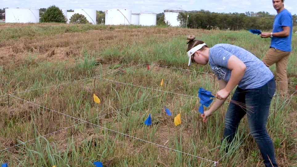
1. Identify sampling zones within a research plot. Determine the number of square grids with equal length (i.e., Figure 1; Figure 3). Based on the size and shape of the research plot, the target number of square grids is expected to be six to ten so that the total number of soil samples is controlled below 30 within a plot (see step 1.3).
2. Mark the center of each square grid (i.e., centroid) and create a circular sampling area with a diameter equal to the side length of the square grid.
3. Stand on the centroid in the circular zone with closed eyes and throw a small stone (or another object with weight) in a random direction and distance from the centroid.
   1. If the stone is dropped outside of the circular area, do it again until the first sampling location is identified.
4. Repeat step 1.3 until three random sampling locations are obtained in the circular zone.
5. Put flags on the three sampling locations and number each flag (i.e., 1, 2, and 3).
6. Repeat steps 1.3 - 1.5 in all other circular sampling zones until all locations are determined and numbered in a sequential order (i.e., 4, 5, 6, etc.).

2. Distance Measurements and Soil Collection in a Plot

1. Choose one corner point and identify it as the origin for the sampling area in the plot.
2. Measure horizontal and vertical distances of each flagged location relative to the origin and record them in a field notebook as x and y coordinates.
3. Use a soil auger to take a soil core (0 - 15 cm) from each flagged location and label the bag based on the flag number. Repeat this step until soil cores are taken at all flagged locations.
4. To minimize the influence of sampling (e.g., trampling on plants and soil in the plot), ensure that the bags with the soil samples inside stay with their respective flag until assembling all bags in the plot at once at the end of the collection.
5. Transport the soil samples in coolers to the laboratory and process each soil core on the same day.
6. Remove roots from each core, sieve it through a 2 mm soil sieve, and thoroughly homogenize each core sample prior to any analysis.
7. Determine soil moisture content in each sample by oven-drying subsamples for 24 h at 105 °C and ground the air-dried soil subsamples to a fine powder for a total carbon (C) analysis using an elemental analyzer⁴. SOC is derived based on the moisture and C contents.
8. Weigh fresh soil subsamples (of 10 g each) and quantify the soil MBC by chloroform fumigation-K₂SO₄ extraction and potassium persulfate digestion methods⁵.
9. Combine the SOC and MBC dataset with x and y coordinates based on the flag numbers in the plot.

3. Descriptive and Geostatistical Analyses in a Plot

1. For each variable of SOC and MBC, calculate the minimum, maximum, mean, median, and standard deviation, as well as the coefficient of variation (CV).
2. For each variable, conduct a set of geospatial analysis (i.e., trend surface analysis, autocorrelation, and kriging map) to depict the primary surface pattern, fine-scale variability, and spatial distribution. The details of the approaches of geostatistical analyses can be found in former publications^4,5.

4. Exploration of SSR and the Associated Sampling Accuracy in a Plot

1. Plot the SSR and relative error (γ) based on the CV obtained in a plot. Within each plot, the log-transformed SSR and relative error (γ) have a negative linear relationship (equations 1 - 3). Based on the relationship (equation 3), the number of samples required for the specified accuracy can be determined:
    
    
   
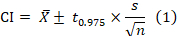
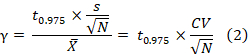
   Here, CI, , s, n, N, CV, and denote the confidence interval, plot mean, plot standard deviation, sample number, coefficient of variation, and relative error, respectively; t_0.975 = 1.96. The log-transformed sample size requirement (N) has a negative linear relationship (i.e., slope = -2) with the log-transformed relative error (γ).
2. Apply the above relationship for future sampling in a plot by calculating N in equation 3 under a desired accuracy (e.g., relative error [γ]). Or, for a given number of soil samples already collected in a plot, apply the relationship to derive at the associated accuracy.

Representative Results

The above approach has been employed in two case studies, one in a Southern US rural region and another in Middle Tennessee.

In the rural Southern Piedmont region, three land-use types were selected, including 1) uncultivated oak-hickory hardwood forests, 2) cultivated fields where conventional tillage and fertilization are used annually to produce wheat, sorghum, and corn, and 3) old-field pine forests that are each about 50 years in age since the last cultivation⁴. Three independently replicated 30 x 30 m plots were identified from the area for each land use. In each plot, a cluster soil sampling design was applied (Figure 1). Each circular zone had a 5 m radial distance from each centroid. Twenty-seven cores were collected from each of the nine plots, 81 cores per land use, and 243 cores in total. SOC was quantified by a CHN analyzer. The major finding was that cultivated land substantially homogenizes the spatial heterogeneity of SOC and other variables⁴. The SSR differed among land uses with a generally ascending order as old-field forest > regenerated pine forest > cultivated cropland (Figure 2). Exceptions are that one hardwood forest plot had an SSR as small as the cultivated plot, and one pine plot had an SSR as large as the hardwood plot (Figure 2). Taking γ = 0.1 or 10% as an example, SSR was 4, 10, and 30 (cultivated cropland), 80, 85, and 300 (pine forest), and 25, 200, and 350 (hardwood). If only three soil samples were collected in all plots, the relative error would have been ~10% - 30% (cultivated cropland), ~50% - 80% (pine forest), and ~28% - 100% (hardwood).

Figure 1: An illustration of a clustered random sampling design within a 30 x 30 m research plot at the Calhoun Experimental Forest, SC, USA⁴. The filled circles represent centroids (n = 9). The large dashed circle represents the sampling area around one centroid (radius = 5 m). Xs represent sample locations determined from randomly chosen directions and distances from a centroid. This figure has been modified from Li et al.⁴. Please click here to view a larger version of this figure.

Figure 2: Plot of the sample size requirement (SSR) and relative error (γ) for SOC of hardwood forest, pine forest, and cultivated cropland. The log scale was applied on both axes. The dotted lines represent cultivated soils, the grey lines pine-forest soils, and the dark lines hardwood forest soils. Three different lines for each land use correspond to three replicate plots. This figure has been modified from Li et al.⁴ Please click here to view a larger version of this figure.

In the Tennessee State University (TSU) Main Campus Agriculture Research and Extension Center (AREC) in Nashville, TN, USA (36.12° N, 36.98° W, elevation 127.6 m) in 2011, a field switchgrass experiment was established with three nitrogen (N) fertilization treatments in a randomized block design⁵. The crop type is of the 'Highlander' variety of eastern 'Alamo' switchgrass (Panicum virgatum L.). The three N treatments included no N fertilizer input (NN), low N fertilizer input (LN: 84 kg of N ha-1 in urea), and high N fertilizer input (HN: 168 kg of N ha-1 in urea). Within each plot, a rectangular area of 2.75 x 5.5 m zone was identified and further divided into eight square grids of 1.375 x 1.375 m. Within each circular zone, a centroid was identified, and three cores were collected with a random direction and distance relative to each centroid (Figure 3). A total of 24 cores were thus collected from each of 12 plots, yielding 288 soil cores. The MBC in each core was quantified by chloroform fumigation-K2SO4 extraction and potassium persulfate digestion methods. The major finding was that the N fertilization generally enhanced the spatial heterogeneity of MBC in the switchgrass cropland. The SSR was generally greater with fertilization (Figure 4). One exception is that the SSR for an HN plot was lower than that of the NN plot (Figure 4). Taking γ = 0.1 or 10% as an example, SSR was 10 and 20 in two replicated plots (NN), 30 and 50 (LN), and 15 and 70 (HN). If only three soil samples were collected in all plots, the relative error would have been ~20% - 25% (NN), ~26% - 35% (LN), and ~20% - 40% (hardwood).

Figure 3: Illustration of a clustered random sampling design within a 2.75 x 5.5 m plot in a fertilization experimental site at the Tennessee State University (TSU) Agricultural Research Center in Nashville, TN, USA. The filled circles represent centroids (n = 8) and each plot consisted of eight centroids in each square grid (of 1.375 x 1.375 m). In each subplot, a circular area was determined for soil sampling. Xs represent sample locations determined from random directions and distances from a centroid within each circular sampling area (dashed circle). This figure has been modified from Li et al.⁵ Please click here to view a larger version of this figure.

Figure 4: Plot of the sample size requirement (SSR) and relative error (γ) for MBC under three fertilization treatments. The log scale was applied on both axes. The dotted lines represent cultivated soils, the grey lines pine-forest soils, and the dark lines hardwood forest soils. NN = no N fertilizer input; LN = low N fertilizer input; and HN = high N fertilizer input. Two different lines for each land use correspond to two replicate plots. This figure has been modified from Li et al.⁵. Please click here to view a larger version of this figure.

Discussion

The traditional soil sampling method lacked a quantitative basis and led to unknown accuracy, whereas the more advanced sampling strategies involved intensive soil collections and induced unaffordable costs for most soil research at the field plot scale. A simple, efficient, and reliable sampling design should be a useful tool to balance both aforementioned methods and, more importantly, inform a quantitative way to determine the number required under certain accuracy for the sake of future sampling needs. However, such a sampling design is still missing. Here, a method for manipulating a clustered sampling procedure to quantify soil spatial heterogeneity was presented and, relying on this design, to inform the number of soil samples required for future sampling under specific accuracy. There are two critical steps within the protocol. The first is to determine the sampling area and identify the sampling zone in a given plot area. Because the dimension and shape of a specific research plot can vary from one study to another, the number and length of the square grid representing the sampling zone should be modified to best fit the plot characteristics and cover the plot area as much as possible. In general, the number of square grids should be limited to eight to ten so that 24 - 30 soil samples will be collected in a given plot. This less intensive sampling requirement is acceptable for a pilot study in a plot. The second critical step is to determine the sample number required under specific accuracy. Although the number of soil samples under a desired accuracy can be derived at based on the pilot sampling strategy, other available resources need to be accounted for (e.g., labor, cost, and personnel). If the number of soil samples required for a desired accuracy exceeds the affordability, the desired accuracy should be lowered so that the number of soil samples can be recalculated. The recalculations should be repeated until the best fit is achieved to balance the desired accuracy and the available resources.

The protocol can be easily modified to fit the specific shape, area, and location of a research plot. Even within an irregular plot or a very large or small plot area, the procedure can be performed by controlling the size of the square grid to cover most of the plot area. On the other hand, when soil samples are collected beyond the circular sampling zone in the plot, they can be still accounted for in the descriptive and geostatistical analysis. The flexibility of the protocol in this regard is advantageous as it can, thus, reduce the cost of sampling.

An important limitation of this method is that the number of soil samples required for certain accuracy will depend upon the plot level CV determined by a group of 24 - 30 soil samples in the pilot soil sampling. For a highly heterogeneous plot, 30 samples or less can produce a larger CV than that based on a greater number of samples (> 30). As a result, the number of soil samples calculated with the same accuracy will be larger. That is, the number of soil samples required for the same accuracy will be overestimated in the plot. For a highly homogenous plot, a smaller number of samples will produce a plot level CV similar to 30 samples, thus, resulting in an overestimation of the resource need. Therefore, for these extremely heterogeneous or homogeneous plots, the soil sample number (i.e., 30 or less) proposed in the pilot sampling design may cause unnecessary investment either in the pilot sampling stage or in future sampling.

We demonstrate significant advantages of the clustered soil sampling strategy. It provides a reliable and affordable soil sampling strategy to obtain soil spatial heterogeneity and offers a quantitative way to derive the number of soil samples required for a certain desired accuracy. Although the intensive strip or stratified sampling may provide a better description of spatial variation, the cost of conducting such sampling is too high for most soil studies. The traditional sampling is arbitrary and lacks any quantitative basis for sampling accuracy. The current protocol is superior due to its less intensive sampling requirement, ease in operating it in the field, power to reveal spatial patterns using rigorous geostatistical analysis methods, and capacity to quantitatively determine the sample size given any desired accuracy. The knowledge of the sample size required for a specific sampling accuracy will allow researchers to strategize their investment in soil sampling efforts.

Employing the efficient clustered sampling procedure allows rigorous testing of soil spatial heterogeneity and improves scientists' capacity to conduct soil sampling with accuracy. The less intensive and quantitative nature of the soil sampling strategy will enable its wide application in soil research communities. Given the likely altered soil spatial heterogeneity under rapid global changes, the soil sample requirement for the same sampling accuracy in a research plot may vary over time. The proposed sample number in the pilot sampling design may vary with different soils and ecosystems. Future applications that could emerge from this work include determining the sample number for specific soils or ecosystems. Thus, further empirical work is needed on the application and identification of the method in various soils and ecosystems. Long-term and wide applications may help identify a generic sample size requirement for specific ecosystems, which can be recommended for soil researchers.

Materials

Name	Company	Catalog Number	Comments
Soil auger	AMS	350.05	For soil collection
Screwdriver	Fisher Scientific	19-313-447	For soil collection
Rope	Fisher Scientific	19-313-429	For delineating sampling zone
FatMax 35 ft. Tape Measure	Home Depot	#215880	For measuring distances
Marking flag	Fisher Scientific	S99537	For marking sampling locations
Plastic Zipper Seal Storage Bag	Fisher Scientific	09-800-16	For soil collection
Sharpie	Fisher Scientific	50-111-3135	For soil collection
Marking pencil	Fisher Scientific	50-294-45	For recording data in field
Lab notebook	Fisher Scientific	11-903	For recording data in field
ArcGis 10.3	ESRI		For producing kriging map
Sieve	Fisher Scientific	04-881G	For sieving soil sample

References

- Young, I. M., Crawford, J. W. Interactions and Self-Organization in the Soil-Microbe Complex. Science. 304 (5677), 1634-1637 (2004).
- Masoom, H., et al. Soil Organic Matter in Its Native State: Unravelling the Most Complex Biomaterial on Earth. Environmental Science and Technology. 50 (4), 1670-1680 (2016).
- Tan, K. Soil Sampling, Preparation, and Analysis. , CRC Press. Boca Raton, FL. (2005).
- Li, J. W., Richter, D. D., Mendoza, A., Heine, P. Effects of land-use history on soil spatial heterogeneity of macro- and trace elements in the Southern Piedmont USA. Geoderma. 156 (1-2), 60-73 (2010).
- Li, J., et al. Nitrogen Fertilization Elevated Spatial Heterogeneity of Soil Microbial Biomass Carbon and Nitrogen in Switchgrass and Gamagrass Croplands. Scientific Reports. 8 (1), 1734 (2018).
- Chung, C. K., Chong, S. K., Varsa, E. C. Sampling Strategies for Fertility on a Stoy Silt Loam Soil. Communications in Soil Science and Plant Analysis. 26 (5-6), 741-763 (1995).
- Luo, Y. Q., et al. Toward more realistic projections of soil carbon dynamics by Earth system models. Global Biogeochemical Cycles. 30 (1), 40-56 (2016).
- Li, J., Wang, G., Allison, S., Mayes, M., Luo, Y. Soil carbon sensitivity to temperature and carbon use efficiency compared across microbial-ecosystem models of varying complexity. Biogeochemistry. 119 (1-3), 67-84 (2014).
- Conant, R. T., Ogle, S. M., Paul, E. A., Paustian, K. Measuring and monitoring soil organic carbon stocks in agricultural lands for climate mitigation. Frontiers in Ecology and the Environment. 9 (3), 169-173 (2011).
- Wieder, W. R., Bonan, G. B., Allison, S. D. Global soil carbon projections are improved by modelling microbial processes. Nature Climate Change. 3 (10), 909-912 (2013).
- Swenson, L. J., Dahnke, W. C., Patterson, D. D. Sampling for Soil Testing. , North Dakota State University, Department of Soil Sciences. Research Report 8 (1984).
- Jones, J. Laboratory Guide for Conducting Soil Tests and Plant Analysis. , CRC Press. Boca Raton, FL. (2001).