Scattering And Absorption of Light in Planetary Regoliths

Summary

Numerical and experimental methods are presented for multiple scattering of light in discrete random media of densely-packed particles. The methods are utilized to interpret the observations of asteroid (4) Vesta and comet 67P/Churyumov-Gerasimenko.

Abstract

Theoretical, numerical, and experimental methods are presented for multiple scattering of light in macroscopic discrete random media of densely-packed microscopic particles. The theoretical and numerical methods constitute a framework of Radiative Transfer with Reciprocal Transactions (R²T²). The R²T² framework entails Monte Carlo order-of-scattering tracing of interactions in the frequency space, assuming that the fundamental scatterers and absorbers are wavelength-scale volume elements composed of large numbers of randomly distributed particles. The discrete random media are fully packed with the volume elements. For spherical and nonspherical particles, the interactions within the volume elements are computed exactly using the Superposition T-Matrix Method (STMM) and the Volume Integral Equation Method (VIEM), respectively. For both particle types, the interactions between different volume elements are computed exactly using the STMM. As the tracing takes place within the discrete random media, incoherent electromagnetic fields are utilized, that is, the coherent field of the volume elements is removed from the interactions. The experimental methods are based on acoustic levitation of the samples for non-contact, non-destructive scattering measurements. The levitation entails full ultrasonic control of the sample position and orientation, that is, six degrees of freedom. The light source is a laser-driven white-light source with a monochromator and polarizer. The detector is a mini-photomultiplier tube on a rotating wheel, equipped with polarizers. The R²T² is validated using measurements for a mm-scale spherical sample of densely-packed spherical silica particles. After validation, the methods are applied to interpret astronomical observations for asteroid (4) Vesta and comet 67P/Churyumov-Gerasimenko (Figure 1) recently visited by the NASA Dawn mission and the ESA Rosetta mission, respectively.

Introduction

Asteroids, cometary nuclei, and airless solar system objects at large are covered by planetary regoliths, loose layers of particles of varying size, shape, and composition. For these objects, two ubiquitous astronomical phenomena are observed at small solar phase angles (the Sun-object-observer angle). First, the brightness of the scattered light in the astronomical magnitude scale is observed to increase nonlinearly toward the zero phase angle, commonly called the opposition effect^1,2. Second, the scattered light is partially linearly polarized parallel to the scattering plane (the Sun-object-observer plane), commonly called negative polarization³. The phenomena have been lacking quantitative interpretation since late 19^th century for the opposition effect and since early 20^th century for the negative polarization. Their proper interpretation is a prerequisite for the quantitative interpretation of the photometric, polarimetric, and spectrometric observations of airless objects, as well as radar scattering from their surfaces.

It has been suggested^4,5,6,7 that the coherent backscattering mechanism (CBM) in multiple scattering is at least partly responsible for the astronomical phenomena. In the CBM, partial waves, interacting with the same scatterers in opposite order, always interfere constructively in the exact backscattering direction. This is due to the coinciding optical paths of the reciprocal waves. In other directions, the interference varies from destructive to constructive. Configurational averaging within a discrete random medium of particles results in enhanced backscattering. As for the linear polarization, the CBM is selective and results in negative polarization in the case of positively polarizing single scatterers, a common characteristic in single scattering (cf. Rayleigh scattering, Fresnel reflection).

Scattering and absorption of electromagnetic waves (light) in a macroscopic random medium of microscopic particles has constituted an open computational problem in planetary astrophysics^8,9. As illustrated above, this has resulted in the absence of quantitative inverse methods to interpret ground-based and space-based observations of solar system objects. In the present manuscript, novel methods are presented for bridging the gap between the observations and their modeling.

Experimental measurements of scattering by a small-particle sample in a controlled position and orientation (six degrees of freedom) has remained open. Scattering characteristics for single particles have been earlier measured as ensemble averages over the size, shape, and orientation distribution¹⁰ by introducing a particle flow through the measurement volume. Scattering characteristics for single particles in levitation have been carried out using, for example, electrodynamic levitation¹¹ and optical tweezers^12,13,14. In the present manuscript, a novel experimental method based on ultrasonic levitation with full control of the sample position and orientation is offered¹⁵.

The present manuscript summarizes the findings of a project funded for five years in 2013-2018 by the European Research Council (ERC): Scattering and Absorption of ElectroMagnetic waves in ParticuLate media (SAEMPL, ERC Advanced Grant). SAEMPL succeeded in meeting its three main goals: first, novel numerical Monte Carlo methods were derived for multiple scattering by discrete random media of densely-packed particles^16,17,18; second, novel experimental instrumentation was developed and constructed for controlled laboratory measurements of validation samples in levitation¹⁵; third, the numerical and experimental methods were applied to interpret astronomical observations^19,20.

In what follows, protocols for utilizing the experimental scattering pipeline for measurements, the corresponding computational pipeline, as well as the application pipelines are described in detail. The computational pipeline consists of software for asymptotically exact computations in the case of finite systems of particles (Superposition T-Matrix Method STMM²¹ and Volume Integral Equation Method VIEM²²) and approximate computations for asymptotically infinite discrete random media of particles using multiple scattering methods (SIRIS^23,24, Radiative Transfer with Coherent Backscattering RT-CB^8,9, and Radiative Transfer with Reciprocal Transactions R²T^{2 16,17,18}). The experimental pipeline encompasses the preparation, storage, and utilization of the samples, their levitation in the measurement volume, and performing the actual scattering measurement across the range of scattering angles with varying polarizer configurations. The application pipeline concerns the utilization of the computational and experimental pipelines in order to interpret astronomical observations or experimental measurements.

Protocol

1. Light scattering measurement

1. Setting up the scatterometer for measurement (Figure 2)
   1. To begin, set up the scatterometer by turning on the light source, photo-multiplier tubes (PMTs), and amplifiers. Allow the system to stabilize for 30 min.
   2. Align and center the incident beam with pinholes. Two pinholes are attached at pre-measured points on the rotating breadboard, 180° apart and at the same radius. Center the beam on the first pinhole and adjust its angle such that the light also enters through the second pinhole.
2. Setting up the acoustic sample levitator
   1. Next, set up the acoustic sample levitator by inserting the microphone in the center of the levitator and running the calibration script.
   2. Calibrate the phased array acoustic levitator by measuring the acoustic pressure for each array element in the intended levitation spot as a function of the driving voltage. Use this calibration to compensate for differences between the array channels. Position the calibration microphone by centering its shadow both in the beam and in a perpendicular beam created with two mirrors.
   3. Calculate the driving parameters for the array that create an asymmetric acoustic trap and supply them to the signal generation electronics. This is accomplished by minimizing the Gor’kov potential²⁵ and aligning the pressure gradients in the levitation spot.
   4. Then, make a measurement sweep with an empty levitator. The sweep reveals any signals generated by ambient light, reflections from the surroundings, or electrical noises.
3. Sample handling, insertion, and measurement
   1. Once set up, use an acoustically transparent mesh spoon to inject the sample into the acoustic levitator.
   2. Using a video camera and high-magnification optics, inspect the orientation and the stability of the sample before and after the scattering measurements.
   3. The strength and asymmetry of the acoustic trap are optimized for maximum sample stability. Consequently, acoustic power is set as low as possible.
   4. If the sample is asymmetric, rotate it around the vertical axis to gain information about its shape. Perform the rotation by slowly changing the alignment of the acoustic trap. While imaging, apply additional illumination to improve the image quality.
   5. Next, close the measurement chamber to block out external light.
   6. Using the computer interface, select the orientation of the sample, as well as the angular resolution and range of the measurement. The incoming and the scattered light are filtered by linear polarizers, which are motorized.
   7. Run the automated measurement sweep. This will measure four points for each angle with polarizer orientations of (horizontal, horizontal), (horizontal, vertical), (vertical, vertical), and (vertical, horizontal).
   8. Repeat each sweep three times to eliminate outliers. For asymmetric samples, repeat the measurement at different sample orientations.
   9. Recover the sample after the measurement by switching off the acoustic field and letting the sample fall on the acoustically transparent fabric. Then, execute another measurement sweep with empty levitator to detect any possible drifting due to the ambient light conditions.
   10. When finished, save the data. Analyze the data to calculate Mueller matrix elements for each angle through linear combination of intensities at different polarizations¹

2. Modeling the mm-sized densely-packed spherical media consisting of spherical particles

1. To begin modeling, use SSH access to connect into the CSC – IT Center for Science Limited’s cluster, Taito.  Download and compile all of the required programs which are preconfigured for Taito by running bash compile.sh.
2. Move into the working directory by executing cd $WRKDIR.
3. Download sources files with git (git clone git@bitbucket.org:planetarysystemresearch/protocol2.git protocol2).
4. Move into the newly created directory cd protocol2.
5. Download and compile required programs by running bash compile.sh, which are preconfigured for Taito.
6. Next, open the text editor nano and set up the parameters for a single scatterer, volume element, and the studied sample to match the studied sample by modifying the file PARAMS.
7. Then, run pipeline by executing a command bash run.sh. When finished, write the full Mueller matrix of the sample into the temp folder as final.out.

3. Interpreting the reflectance spectra for asteroid (4) Vesta

1. Deriving the complex refractive indices for howardite.
   1. Download SIRIS4 (git clone git@bitbucket.org:planetarysystemresearch/siris4.2.git).
   2. Compile by executing make in the src-folder. Rename the executable siris42 to siris4.
   3. In mainGo.f90, change line 395 to r0=0.05*rmax*sqrt(ran2). Compile by executing make.
   4. Download the needed MATLAB scripts by executing “git clone git@bitbucket.org:planetarysystemresearch/protocol4a.git”.
   5. Copy the executable files created in steps 3.1.2. and 3.1.3. to JoVEOptimize-folder.
   6. Go to folder JoVEOptimize.
   7. In input1.in file, set the radius to 30 µm for the howardite particle size, and fix the real part of the refractive index to 1.8. In input2.in file, set the radius to 15,000 µm.
   8. Estimate the upper and lower boundaries for the imaginary part of the refractive indices and save them into two separate files. The code utilizes the bisectioning method and uses these values as the starting point.
   9. In optimizek.m file, set the file names of the upper and lower boundaries of the imaginary part of the refractive indices and the file name of the measured reflectance spectrum of the howardite powder. Set the wavelength range to 0.4–2.5 µm with 0.05-µm steps.
   10. Run optimizek.m in MATLAB to obtain the complex refractive indices for howardite (see Figure 3). First, the code computes scattering properties for 30-µm sized (radius) howardite particles, and then uses these particles as diffuse scatterers inside a 15,000-µm sized (radius) volume. These steps are repeated for each wavelength until the computed reflectance matches with the measured reflectance.
2. Modeling the reflectance spectrum of Vesta.
   1. Computing the scattering properties of howardite particles by utilizing SIRIS4
      1. Utilize SIRIS4 to compute the scattering properties of howardite particles by first moving the siris4 executable file into the same folder with the input-file and p-matrix-file.  Then, copy the input_1.in and pmatrix_1.in from the test-folder.
      2. In input_1.in, set the number of rays to 2 million, the number of sample particles to 1000, the standard deviation of radius to 0.17, and the power-law index of the correlation function to 3. Then, set the real part of the refractive index to 1.8 and use the imaginary part of the refractive index n as described in the text protocol.
      3. Next, run SIRIS4 by executing the command shown here for each wavelength from 0.4 to 2.5 microns using a size range of 10 to 200 microns in diameter with a sampling step of 10 microns.
      4. Next, save each computed scattering phase matrix P into a pmatrix_x.in file.  The x in the file name describes the wavelength number and ranges from 1 to 43 for each particle size. The file will contain the scattering angles as well as the scattering matrix elements P₁₁, P₁₂, P₂₂, P₃₃, P₃₄, and P₄₄ for one wavelength and particle size.
   2. Average the obtained scattering matrices, single-scattering albedos, and mean-free paths over a power-law size distribution with an index of 3.2^19,24.
      1. Move the pmatrix-files into folders so that each folder represents one particle size and contains the computed p-matrices for all the wavelengths. Name the folders fold1, fold2,…, foldN, where N is the number of particle sizes.
      2. Write the scattering and extinction efficiencies q_sca and q_ext, as well as the equal-projected-area-sphere radius values r_hit from the outputQ-files into one file, Qscas.dat.
      3. Go to folder JoVEAverage that was downloaded in step 3.1.4.
      4. Move the folders and Qscas.dat into the same folder with AvgPowerLaw.m.
      5. Run AvgPowerLaw.m in MATLAB. The code computes averaged scattering matrices, single-scattering albedos, and mean free- path lengths over a power-law size distribution with index 3.2.
   3. Computing the final spectrum of Vesta by utilizing SIRIS4
      1. Use diffuse scatterers inside a Vesta-sized volume with a refractive index of 1. In the input-file, use the averaged single-scattering albedos and mean free path lengths for internal scatterers.
      2. Next, run SIRIS4 at each wavelength by executing the command shown here, where X is the wavelength. The code reads the averaged scattering matrices as its input for the internal diffuse scatterers.
      3. Study the absolute reflectance at a 17.4-degree phase angle.
      4. Obtain Vesta’s observed spectra at 17.4-degree phase angle from the NASA Planetary Data System²⁶.
      5. Scale Vesta’s observed spectra to a geometric albedo value of 0.42327 at 0.55 microns²⁷. To get to 17.4 degrees, apply a factor of 0.491 on the scaled spectra²⁸. Compare both the modeled and the observed spectra across the whole wavelength range.

4. Photometric and polarimetric modeling of (4) Vesta

1. Computing scattering properties for volume elements containing Voronoi-shaped howardite particles
   1. Connect into the CSC – IT Center for Science Ltd.’s cluster Taito via SSH access.
   2. Move into the working directory by executing cd $WRKDIR.
   3. Download the source files (git clone git@bitbucket.org:planetarysystemresearch/jvie_t_matrix.git).
   4. Compile by executing make in the -folder.
   5. Generate volume elements that contain Voronoi-shaped howardite particles by using a MATLAB-code voronoi_element.m. In voronoi_element.m, set the wavelength to 0.45 µm, N_elems to 128, the size parameter (elem_ka) to 10, power-law index to 3, minimum particle radius to 0.143 µm, maximum particle radius to 0.35 µm, packing density to 30%, and use the derived complex refractive index for howardite.
   6. Run voronoi_element.m in MATLAB. The code generates 128 mesh-files for volume-elements with different Voronoi-particle realizations using the power-law size distribution.
   7. Compute T-matrices for the generated volume-elements by using JVIE. In runarray_JVIE_T.sh, set array=1-128. The paramaters are k = 13.962634, mesh = name of the generated mesh in 4.1.6, T_out = name of the output T-matrix, T_matrix = 1, and elem_ka = 10.
   8. Run JVIE by executing sbatch runarray_JVIE_T.sh.
   9. Compute averaged scattering properties from the T-matrices computed with the JVIE code. Execute ./multi_T -N_Tin 128 in the same folder where the computed T-matrices are. The code writes the averaged incoherent Mueller matrix into and the cross-sections and albedo into output.txt.
2. RT-CB computations
   1. Start by downloading the sources files with git (git clone git@bitbucket.org:planetarysystemresearch/protocol4b.git protocol4b) and move the files into the downloaded directory protocol4b.
   2. Next, download and compile all of the required programs by running bash compile.sh.
   3. When ready, copy the averaged input scattering matrix (step 3.2.2.5) as well as the amplitude scattering matrix (step 4.1.9) into the current working directory.
   4. Next, open the text editor, nano, and modify the file PARAMS to set the desired parameters.
   5. Run the pipeline by executing bash run.sh. Then, write the full Mueller matrix into the temp folder as rtcb.out.

5. Interpreting the observations for Comet 67P/Churyumov-Gerasimenko.

1. Computing incoherent volume elements with the fast superposition T-matrix method (FaSTMM) for the organic and particle grains
   1. Execute ./incoherent_input –lambda 0.649 -m_r 2.0 -m_i 0.2 -density 0.3 -lowB 0.075 -upB 0.125 -npower 3 -S_out pmatrix_org.dat.
   2. Execute ./incoherent_input –lambda 0.649 -m_r 1.6 -m_i 0.0001 -density 0.0375 -lowB 0.6 -upB 1.3 -npower 3 -S_out pmatrix_sil.dat.
2. Computing the average incoherent Mueller matrix (pmatrix.in), albedo (albedo), mean free path (mfp), and coherent effective refractive index (m_eff)
   1. Run matlab. Type commands:
      Sorg=load('pmatrix_org.dat');
      Ssil=load('pmatrix_sil.dat');
      S = (Sorg+Ssil)/2; save('pmatrix.in','S','-ascii');
      Csca = (Csca_sil + Csca_org)/2;
      Cext = (Cext_sil + Cext_org)/2;
      albedo = Csca/Cext;
      mfp = Vol/Cext;
      where Csca_org and Cext_org are the incoherent scattering and extinction cross sections from the step 5.1.2, and Csca_sil and Cext_sil are the incoherent scattering and extinction cross sections from the step 5.1.3.
   2. Run ./m_eff(Csca, r) in the command line to obtain m_eff where is the radius of the volume element.
3. Computing scattering properties for the coma particles.
   1. Set the values from the step 5.2.1 and 5.2.2 (i.e., albedo, mfp, m_eff in the input.in file).
   2. Set power-law index for the correlation length to 3.5 in the input.in file.
   3. Run SIRIS4 solver (./siris4 input.in pmatrix.in) for particle sizes from 5 µm to 100 µm using a step of 5.
   4. Output the coma phase functions from the SIRIS4 solver.
4. Computing scattering properties of the nucleus
   1. Start in MATLAB and run the averaging routine powerlaw_ave.m to average the results over the power-law size distribution of index -3 after calculating the coma phase functions (step 5.3.4) from the SIRIS4 solver. The expected routine outputs are pmatrix2.in, albedo, and the mean free path.
   2. Next, set the results from the outputs, albedo and the mean free path, into the input.in file. 
   3. Set the size to 1 billion, and the power-law index of the correlation function for the shape to 2.5. Then, run SIRIS4 using the command line shown here to obtain the nucleus phase function.

Representative Results

For our experiment, an aggregate nominally consisting of densely-packed Ø=0.5 µm spherical SiO₂ particles was selected^29,30 and polished further, to approximate a spherical shape, after which it was characterized by weighing and measuring its dimensions (Figure 4). The nearly spherical aggregate had a diameter of 1.16 mm and a volume density of 0.47. Light scattering was measured according to step 1. The beam was filtered to 488±5 nm, with a Gaussian spectrum. The measurement was averaged from three sweeps and the empty levitator signal was subtracted from the result.

From the intensities of the four different polarization configurations, we calculated the phase function, the degree of linear polarization for unpolarized incident light -M₁₂/M₁₁, and the depolarization M₂₂/M₁₁, as a function of the phase angle (Figure 5, Figure 6, Figure 7). One known systematic error source of our measurement is the extinction ratio of the linear polarizers, which is 300:1. For this sample, it is, however, adequate so that the leaked polarized light is below the detection threshold.

The numerical modeling consists of multiple software interlinked by scripts which handle the information flow according to the parameters given by the user. The scripts and software are preconfigured to work on the CSC - IT Center for Science Ltd.’s Taito cluster, and the user needs to modify the scripts and Makefiles themselves to get the modeling tool to work on other platforms. The tool starts by running the STMM solver²⁰, which computes volume-element characteristics as described by Väisänen et al.¹⁸. After that, the scattering and absorption characteristics of the volume element are used as input for two different software. A Mie-scattering solver is used to find the effective refractive index by matching the coherent scattering cross section of the volume element to a Mie sphere of equal size²⁰. Then the aggregate is modeled by running the SIRIS4 software with the volume element as a diffuse scatterer and with the effective refractive index on the surface of the aggregate. The coherent backscattering component is added separately because there is no software that can treat effective refractive medium and coherent backscattering simultaneously. Currently, the RT-CB is incapable of accounting for the effective refractive medium, whereas the SIRIS4 is incapable of accounting for coherent backscattering. The coherent backscattering is, however, added to the SIRIS4^23,24 results approximately by running the volume-element scattering characteristics through the scattering phase matrix decomposition software PMDEC which derives pure Mueller and Jones matrices required for the RT-CB⁹. The coherent backscattering component is then extracted by subtracting the radiative transfer component from the results of the RT-CB. Then, the extracted coherent backscattering component is added to the results obtained from the SIRIS4.

We simulated numerically the properties of the mm-sized (radius 580 µm) SiO₂ aggregate by following step 2. We used two kinds of volume elements, one consisting of nominal equisized particles (0.25 µm) and the other consisting of normally distributed (mean 0.25 µm, standard deviation 0.1 µm) particles truncated to the range of 0.1-0.2525 µm. Introducing the latter distribution of particles is based on the fact that essentially all SiO₂ samples with a given nominal particle size also have a significant alien distribution of smaller particles³¹. In total, 128 volume elements of size kR₀=10 were drawn from 128 periodic boxes containing about 10,000 particles packed to the volume density v=47 % each. From the specifications of the material, we have n=1.463+i0 at the wavelength of 0.488 µm, which is the wavelength used in the measurements.

With SIRIS4, the scattering properties of 100,000 aggregates, with radius of 580 µm, standard deviation of 5.8 µm, and with the power-law index of the correlation function 2, were solved and averaged. These results are plotted (see Figure 5, Figure 6, Figure 7) with the experimental measurements, and an additional simulation without the effective medium. Both choices for the particle distribution produce a match to the measured phase function (see Figure 5), although they result in different polarization characteristics as is seen in Figure 6. These differences can be used to identify the underlying distribution of the particles in the sample. The best choice is to use the truncated normal distribution instead of the equisized particles (see Figure 6). If only normalized phase functions are used, the underlying distributions are indistinguishable (compare Figure 5, Figure 6, Figure 7). In Figure 7 for the depolarization, the numerical results have features similar to the measured curve, but the functions are shifted by 10° to the backscattering direction. The effective refractive index positively corrects the results as is seen from the simulations obtained with and without the effective medium (see Figure 5, Figure 6, Figure 7). The differences in the polarization (Figure 6) indicate that the sample has presumably a more complex structure (e.g., a separate mantle and core) than our homogeneous model. It is, however, beyond the existing microscopic methods for sample characterization to retrieve the true structure of the aggregate. The coherent backscattering was added separately to the results. The measurements lack visible intensity spike observed at the backscattering angles, but the degree of linear polarization is more negative between 0-30° which cannot be produced without coherent backscattering (compare “distribution” with “no cb”, see Figure 5, Figure 6, Figure 7).

For solar system applications, we compared the observed Vesta spectra and the modeled spectrum obtained by following protocol 3. The results are shown in Figure 3 and Figure 8 and they suggest that howardite particles, with more than 75% of them having a particle size smaller than 25 µm, dominate Vesta’s regolith. Although the overall match is quite satisfactory, the modeled and observed spectra differ slightly: the absorption band centers of the model spectrum are shifted to longer wavelengths, and the spectral minima and maxima tend to be shallow as compared to the observed spectra. The differences in the minima and maxima could be explained by the fact that mutual shadowing effects among the regolith particles have not been accounted for: the shadowing effects are stronger for low reflectances and weaker for high reflectances and, in the relative sense, would decrease the spectral minima and increase the spectral maxima when accounted for in the modeling. Furthermore, the imaginary part of the complex refractive indices for howardite was derived without taking into account wavelength-scale surface-roughness, and thus the derived values can be too small to explain the spectral minima. When further using these values in our model by utilizing geometric optics, the band depths in the modeled spectrum can become too shallow. These wavelength-scale effects could also play a part at longer wavelengths together with a small contribution from the low-end tail of the thermal emission spectrum. The differences can also be caused by a compositional mismatch of our howardite sample and Vesta minerals and by a different particle size distribution needed for the model. Finally, the reflectance spectra of Vesta were observed at 180-200 K, and our howardite sample was measured in room temperature. Reddy et al.³² have shown that the absorption band centers shift to longer wavelengths with increasing temperature.

The photometric and polarimetric phase curve observations for asteroid (4) Vesta are from Gehrels³³ and the NASA Planetary Data System’s Small Bodies Node (http://pdssbn.astro. umd.edu/sbnhtml), respectively. Their modeling follows step 4 and starts from the particle refractive index and size distribution available from the spectrometric modeling at the wavelength of 0.45 µm. These particles have sizes larger than 5 µm, that is, much larger than the wavelength and are thus in the geometric optics regime, termed large-particle population. For the phase curve modeling, an additional small-particle population of densely-packed subwavelength-scale particles is also incorporated, with due attention paid to avoid conflicts with the spectrometric modeling above.

The complex refractive index has been set to 1.8+i0.000168. The effective particle sizes and single-scattering albedos in the large-particle and small-particle populations equal (9.385 µm, 0.791) and (0.716 µm, 0.8935), respectively. The mean free path lengths in the large-particle and small-particle media are 16.39 µm and 0.56 µm. The large-particle medium has a volume density of 0.4, whereas the small-particle medium has a volume density of 0.3. The fractions of large-particle and small-particle media in the Vesta regolith are assumed to be 99% and 1%, respectively, giving a total single-scattering albedo of 0.815 and a total mean free path length of 12.78 µm. Following step 4, the Vesta geometric albedo at 0.45 µm turns out to be 0.32 in fair agreement with the observations (cf. Figure 8 when extrapolated to zero phase angle).

Figure 9, Figure 10, Figure 11 depict the photometric and polarimetric phase curve modeling for Vesta. For the photometric phase curve (Figure 10, left), the model phase curve from RT-CB has been accompanied with a linear dependence on the magnitude scale (slope coefficient -0.0179 mag/°), mimicking the effect of shadowing in a densely-packed, high-albedo regolith. No alteration has been invoked for the degree of polarization (Figure 10, right; Figure 11). The model successfully explains the observed photometric and polarimetric phase curves and offers a realistic prediction for the maximum polarization near the phase angle of 100° as well as for the characteristics at small phase angles <3°.

It is striking how the minute fraction of the small-particle population is capable of completing the explanation of the phase curves (Figure 10, Figure 11). There are intriguing modeling aspects involved. First, as shown in Figure 9 (left), the single-scattering phase functions for the large-particle and small-particle populations are quite similar, whereas the linear polarization elements are significantly different. Second, in the RT-CB computations, both particle populations contribute to the coherent backscattering effects. Third, in order to obtain realistic polarization maxima, there has to be a significant large-particle population in the regolith (in agreement with the spectral modeling). With the current independent mixing of the small-particle and large-particle media, it remains possible to assign a part of the small-particle contribution to the large-particle surfaces. However, in order for coherent backscattering effects to take place and to explain the observations, it is obligatory to incorporate a small-particle population.

The European Space Agency’s (ESA) Rosetta mission to the comet 67P/Churyumov-Gerasimenko provided an opportunity to measure the photometric phase function of the coma and the nucleus over a wide phase-angle range within just a few hours³⁴. The measured coma phase functions show a strong variation with time and a local position of the spacecraft. The coma phase function has been successfully modeled²⁰ with a particle model composed of submicrometer-sized organic and silicate particles using the numerical methods (steps 5 and 2) as shown in Figure 12. The results suggest that the size distribution of dust varies in the coma due to the comet’s activity and the dynamical evolution of the dust. By modeling scattering by a 1-km-sized object whose surface is covered with the dust particles, we have shown that scattering by the nucleus of the comet is dominated with the same type of particles that also dominate the scattering in the coma (Figure 13).

Figure 1: Asteroid (4) Vesta (left) and Comet 67P/Churyumov-Gerasimenko (right) visited by the NASA Dawn mission and by the ESA Rosetta mission, respectively. Image credits: NASA/JPL/MPS/DLR/IDA/Björn Jónsson (left), ESA/Rosetta/NAVCAM (right). Please click here to view a larger version of this figure.

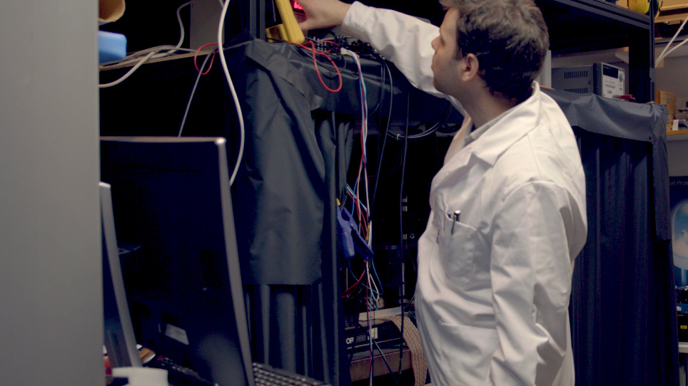
Figure 2: Light scattering measurement instrument. Photo (above) and top view schematic (below) showing: (1) fiber-coupled light source with collimator, (2) focusing lens (optional), (3) bandpass filter for wavelength selection, (4) adjustable aperture for beam shaping, (5) motorized linear polarizer, (6) high-speed camera, (7) high-magnification objective, (8) acoustic levitator for sample trapping, (9) measurement head, comprising an IR filter, motorized shutter, motorized linear polarizer, and a photomultiplier tube (PMT), (10) motorized rotation stage for adjusting measurement head angle, (11) optical flat for Fresnel reflection, (12) neutral density filter, and (13) reference PMT, for monitoring beam intensity. The system is divided into three enclosed compartments to eliminate stray light. Please click here to view a larger version of this figure.

Figure 3: The imaginary part of the refractive index for howardite as a function of wavelength. The imaginary part of the refractive Im(n) obtained for the howardite mineral by following protocol 3.1. The refractive index is utilized in modeling the scattering characteristics of asteroid (4) Vesta. Please click here to view a larger version of this figure.

Figure 4: The measurement sample composed of densely-packed spherical SiO₂ particles. The sample has been carefully polished in order to obtain a nearly spherical shape that allows for both efficient scattering experiments and numerical modeling. Please click here to view a larger version of this figure.

Figure 5: Phase function. The phase functions of the sample aggregate obtained by following the experimental protocols 1 and the numerical modeling step 2. The phase functions are normalized to give unity when integrated from 15.1° to 165.04°. Please click here to view a larger version of this figure.

Figure 6: Degree of linear polarization. As in Figure 5 for the degree of linear polarization for unpolarized incident light -M₁₂/M₁₁ (in %). Please click here to view a larger version of this figure.

Figure 7: Depolarization. As in Figure 5 for the depolarization M₂₂/M₁₁. Please click here to view a larger version of this figure.

Figure 8: Absolute reflectance spectra. Asteroid (4) Vesta’s modeled and observed absolute reflectance spectra at 17.4-degree phase angle. Please click here to view a larger version of this figure.

Figure 9: Scattering phase function P₁₁ and degree of linear polarization for unpolarized incident light -P₂₁/P₁₁ as a function of the scattering angle for volume elements of large particles (red) and small particles (blue) in the regolith of asteroid (4) Vesta. The dotted line indicates a hypothetical isotropic phase function (left) and a zero level of polarization (right). Please click here to view a larger version of this figure.

Figure 10: Observed (blue) and modeled (red) disk-integrated brightness in the magnitude scale as well as the degree of linear polarization for unpolarized incident light as a function of phase angle for asteroid (4) Vesta. The photometric and polarimetric observations are from Gehrels (1967) and the Small Bodies Node of the Planetary Data System (http://pdssbn.astro.umd.edu/sbnhtml), respectively. Please click here to view a larger version of this figure.

Figure 11: Degree of linear polarization. The degree of linear polarization for asteroid (4) Vesta predicted for large phase angles based on the numerical multiple-scattering modeling. Please click here to view a larger version of this figure.

Figure 12: Modeled and measured photometric phase functions in the coma of comet 67P/Churyumov-Gerasimenko. The variations in the measured phase functions in time can be explained by varying dust size distribution in the coma. Please click here to view a larger version of this figure.

Figure 13: Phase functions. Modeled and measured phase functions of the nucleus of comet 67P. Please click here to view a larger version of this figure.

Discussion

Experimental, theoretical, and computational methods have been presented for light scattering by discrete random media of particles. The experimental methods have been utilized to validate the basic concepts in the theoretical and computational methods. The latter methods have then been successfully applied in the interpretation of astronomical observations of asteroid (4) Vesta and comet 67P/Churyumov-Gerasimenko.

The experimental scatterometer relies on ultrasonically controlled sample levitation that allows for Mueller-matrix measurements for a sample aggregate in a desired orientation. The aggregate can be repeatedly utilized in the measurements, as it is possible to conserve the aggregate after each measurement set. This is the first time that such non-contact, non-destructive scattering measurements are carried out on a sample under full control.

The theoretical and computational methods rely on the so-called incoherent scattering, absorption, and extinction processes in random media. Whereas the exact electromagnetic interactions always occur coherently, within an infinite random medium after configurational averaging, only incoherent interactions remain among volume elements of particles. In the present work, the incoherent interactions among these elements are exactly accounted for by using the Maxwell equations: after subtracting the coherent fields from the fields in free space, it is the incoherent fields within the random medium that remain. The treatment has presently been taken to its complete rigor in that the interactions, as well as the extinction, scattering, and absorption coefficients of the medium, are derived within the framework of incoherent interactions. Furthermore, it has been shown that accounting for the coherent field effects on the interface between the free space and the random medium results in a successful overall treatment for a constrained random medium.

Application of the theoretical and computational methods has been illustrated for experimental measurements of a mm-scale spherical sample aggregate composed of submicron-scale spherical SiO₂ particles. The application shows, unequivocally, that the sample aggregate must be composed of a distribution of particles with varying sizes, instead of being composed of equisized spherical particles. There may be far-reaching consequences of this result for the characterization of random media: it is plausible that the media are significantly more complex than what has been deduced earlier using state-of-the-art characterization methods.

The synoptic interpretation of the spectrum for asteroid (4) Vesta across the visible and near-infrared wavelengths as well as Vesta’s photometric and polarimetric phase curves at the wavelength of 0.45 µm shows that it is practical to utilize the numerical methods in constraining the mineral compositions, particle size distributions, as well as regolith volume density from remote astronomical observations. Such retrievals are further enhanced by the simultaneous interpretation of the photometric phase curves for comet 67P/Churyumov-Gerasimenko concerning its coma and nucleus. Finally, realistic modeling of the polarimetric phase curve of 67P has been obtained²⁰. There are major future prospects in applying the present methods in the interpretation of observations of solar system objects at large.

There are future prospects for the present combined experimental and theoretical approach. As it is extremely difficult to accurately characterize random media composed of sub-wavelength-scale inhomogeneities, controlled Mueller-matrix measurements can offer a tool for retrieving information on the volume density and particle size distribution in the medium. Quantitative inversion of these physical parameters is facilitated by the novel numerical methods.

Materials

Name	Company	Catalog Number	Comments
10GL08	Newport		Calcite polarizer
12X Zoom Body Tube 1-50487AD	Navitar		Microscope objective
43-412-000	Edmund optics		Optical flat
8MPR16-1	Standa		Motorized Polarizer Rotator
8MRB240-152-59D	Standa		Rotation stage
8SMC5-ETHERNET	Standa		Motor controller
Digi-pas DWL3500XY	Digi-pas		Digital 2-axis level
DMT 65-D25-HiDS	Owis		Optics rotation stage
EQ-99 LDLS	Energetiq		Light source
FL488-10	Thorlabs		Laser line filter
IBM 65-D0-35-HiDS	Owis		Motorized iris shutter
LPVISE100-A	Thorlabs		Film polarizer
microPMT H12403-01	Hamamatsu		Photomultiplier tube
NI PXIe-5171R	National Instruments		Digital oscilloscope
NI PXIe-8880	National Instruments		PXIe chassis
Phantom v611	Vision Research		High speed camera
PS 10-32-DC	Owis		Motor controller
RC08FC-P01	Thorlabs		Fiber collimator
SET-NDF-D22-G25	Owis		Neutral density filter
TIA60	Thorlabs		PMT amplifier

References

- Gehrels, T. Photometric studies of asteroids. V. The light-curve and phase function of 20 Massalia. Astrophysical Journal. 123, 331-338 (1956).
- Barabashev, N. P. Astronomische Nachrichten. 217, 445 (1922).
- Lyot, B. Recherches sur la polarisation de la lumiere des planetes et de quelques substances terrestres. Annales de l’Observatoire de Paris. 8 (1), 1-161 (1956).
- Shkuratov, Y. G. Diffractional model of the brightness surge of complex structures. Kinematika i fizika nebesnyh tel. 4, 60-66 (1988).
- Shkuratov, Y. G. A new mechanism of the negative polarization of light scattered by the surfaces of atmosphereless celestial bodies. Astronomicheskii vestnik .23. , 176-180 (1989).
- Muinonen, K. Electromagnetic scattering by two interacting dipoles. Proceedings of the 1989 URSI Electromagnetic Theory Symposium. , Stockholm. 428-430 (1989).
- Muinonen, K. Light Scattering by Inhomogeneous Media: Backward Enhancement and Reversal of Polarization. , PhD-thesis, University of Helsinki, Finland. (1990).
- Muinonen, K., Mishchenko, M. I., Dlugach, J. M., Zubko, E., Penttilä, A., Videen, G. Coherent backscattering numerically verified for a finite volume of spherical particles. Astrophysical Journal. 760, 118-128 (2012).
- Muinonen, K. Coherent backscattering of light by complex random media of spherical scatterers: Numerical solution. Waves in Random Media. 14, 365-388 (2004).
- Muñoz, O., Volten, H., de Haan, J. F., Vassen, W., Hovenier, J. W. Experimental determination of scattering matrices of olivine and Allende meteorite particles. Astronomy & Astrophysics. 360, 777-788 (2000).
- Sasse, C., Muinonen, K., Piironen, J., Dröse, G. Albedo measurements on single particles. Journal of Quantitative Spectroscopy and Radiative Transfer. 55, 673-681 (1996).
- Gong, Z., Pan, Y. -L., Videen, G., Wang, C. Optical trapping and manipulation of single particles in air: Principles, technical details, and applications. Journal of Quantitative Spectroscopy and Radiative Transfer. 214, 94-119 (2018).
- Nieminen, T. A., du Preez-Wilkinson, N., Stilgoe, A. B., Loke, V. L. Y., Bui, A. A. M., Rubinsztein-Dunlop, H. Optical tweezers: Theory and modelling. Journal of Quantitative Spectroscopy and Radiative Transfer. 146, 59-80 (2014).
- Herranen, J., Markkanen, J., Muinonen, K. Dynamics of interstellar dust particles in electromagnetic radiation fields: A numerical solution. Radio Science. 52 (8), 1016-1029 (2017).
- Maconi, G., et al. Non-destructive controlled single-particle light scattering measurement. Journal of Quantitative Spectroscopy and Radiative Transfer. 204, 159-164 (2018).
- Muinonen, K., Markkanen, J., Väisänen, T., Peltoniemi, J., Penttilä, A. Multiple scattering of light in discrete random media using incoherent interactions. Optics Letters. 43, 683-686 (2018).
- Markkanen, J., Väisänen, T., Penttilä, A., Muinonen, K. Scattering and absorption in dense discrete random media of irregular particles. Optics Letters. 43, 2925-2928 (2018).
- Väisänen, T., Markkanen, J., Penttilä, A., Muinonen, K. Radiative transfer with reciprocal transactions: Numerical method and its implementation. Public Library of Science One (PLoS One). 14, e0210155 (2019).
- Martikainen, J., Penttilä, A., Gritsevich, M., Videen, G., Muinonen, K. Absolute spectral modelling of asteroid (4). Monthly Notices of the Royal Astronomical Society. 483, 1952-1956 (2019).
- Markkanen, J., Agarwal, J., Väisänen, T., Penttilä, A., Muinonen, K. Interpretation of phase functions of the comet 67P/Churyumov-Gerasimenko measured by the OSIRIS instrument. Astrophysical Journal Letters. 868 (1), L16 (2018).
- Markkanen, J., Yuffa, A. J. Fast superposition T-matrix solution for clusters with arbitrarily-shaped constituent particles. Journal of Quantitative Spectroscopy and Radiative Transfer. 189, 181-188 (2017).
- Markkanen, J., Ylä-Oijala, P. Numerical Comparison of Spectral Properties of Volume-Integral-Equation Formulations. Journal of Quantitative Spectroscopy and Radiative Transfer. 178, 269-275 (2016).
- Lindqvist, H., Martikainen, J., Räbinä, J., Penttilä, A., Muinonen, K. Ray optics for absorbing particles with application to ice crystals at near-infrared wavelengths. Journal of Quantitative Spectroscopy and Radiative Transfer. 217, 329-337 (2018).
- Martikainen, J., Penttilä, A., Gritsevich, M., Lindqvist, H., Muinonen, K. Spectral modeling of meteorites at UV-vis-NIR wavelengths. Journal of Quantitative Spectroscopy and Radiative Transfer. 204, 144-151 (2018).
- Gor'kov, L. P. On the forces acting on a small particle in an acoustical field in an ideal fluid. Soviet Physics Doklady. 6, (1962).
- Reddy, V. Vesta Rotationally Resolved Near-Infrared Spectra V1.0. EAR-A-I0046-3-REDDYVESTA-V1.0. NASA Planetary Data System. , (2011).
- Tedesco, E. F., Noah, P. V., Noah, M., Price, S. D. IRAS Minor Planet Survey. IRAS-A-FPA-3-RDR-IMPS-V6.0. NASA Planetary Data System. , (2004).
- Hicks, M. D., Buratti, B. J., Lawrence, K. J., Hillier, J., Li, J. -Y., Vishnu Reddy, V., Schröder, S., Nathues, A., Hoffmann, M., Le Corre, L., Duffard, R., Zhao, H. -B., Raymond, C., Russell, C., Roatsch, T., Jaumann, R., Rhoades, H., Mayes, D., Barajas, T., Truong, T. -T., Foster, J., McAuley, A. Spectral diversity and photometric behavior of main-belt and near-Earth vestoids and (4) Vesta: A study in preparation for the Dawn encounter. Icarus. 235, 60-74 (2014).
- Weidling, R., Güttler, C., Blum, J. Free collisions in a micro-gravity many-particle experiment. I. Dust aggregate sticking at low velocities. Icarus. 218, 688-700 (2012).
- Blum, J., Beitz, E., Bukhari, M., Gundlach, B., Hagemann, J. -H., Heißelmann, D., Kothe, S., Schräpler, R., von Borstel, I., Weidling, R. Laboratory drop towers for the experimental simulation of dust-aggregate collisions in the early solar system. Journal of Visualized Experiments (JoVE). (88), e51541 (2014).
- Poppe, T., Schräpler, R. Further experiments on collisional tribocharging of cosmic grains. Astronomy & Astrophysics. 438, 1-9 (2005).
- Reddy, V., Sanchez, J. A., Nathues, A., Moskovitz, N. A., Li, J. -Y., Cloutis, E. A., Archer, K., Tucker, R. A., Gaffey, M. J., Mann, J. P., Sierks, H., Schade, U. Photometric spectral phase and temperature effects on Vesta and HED meteorites: Implications for Dawn mission. Icarus. 217, 153-168 (2012).
- Gehrels, T. Minor planets. I. The rotation of Vesta. Photometric studies of asteroids. Astronomical Journal. 72, 929-938 (1967).
- Bertini, I., La Forgia, F., Tubiana, C., Güttler, C., Fulle, M., Moreno, F., Frattin, E., Kovacs, G., Pajola, M., Sierks, H., Barbieri, C., Lamy, P., Rodrigo, R., Koschny, D., Rickman, H., Keller, H. U., Agarwal, J., A'Hearn, M. F., Barucci, M. A., Bertaux, J. -L., Bodewits, D., Cremonese, G., Da Deppo, V., Davidsson, B., Debei, S., De Cecco, M., Drolshagen, E., Ferrari, S., Ferri, F., Fornasier, S., Gicquel, A., Groussin, O., Gutierrez, P. J., Hasselmann, P. H., Hviid, S. F., Ip, W. -H., Jorda, L., Knollenberg, J., Kramm, J. R., Kührt, E., Küppers, M., Lara, L. M., Lazzarin, M., Lin, Z. -Y., Lopez Moreno, J. J., Lucchetti, A., Marzari, F., Massironi, M., Mottola, S., Naletto, G., Oklay, N., Ott, T., Penasa, L., Thomas, N., Vincent, J. -B. The scattering phase function of comet 67P/Churyumov-Gerasimenko coma as seen from the Rosetta/OSIRIS instrument. Monthly Notices of the Royal Astronomical Society. 469, 404-415 (2017).