Is My Mouse Pregnant? High-Frequency Ultrasound Assessment

Summary

High-resolution ultrasound can help streamline experiments requiring timed-pregnant mice by determining the state of pregnancy, gestational age, and pregnancy losses. Presented here is a protocol to illustrate methods to assess mouse pregnancies as well as potential pitfalls (image artifacts) that may mimic pregnancy.

Abstract

The mouse is the mammalian animal model of choice for many human diseases and biological processes. Developmental biology often requires staged-pregnant mice to determine evolving processes at various timepoints. Moreover, optimal and efficient breeding of model mice requires an assessment of timed pregnancies. Most commonly, mice are mated overnight, and the presence of a vaginal plug is determined; however, the positive predictive value of this technique is suboptimal, and one needs to wait to know if the mouse is truly pregnant. High-resolution ultrasound biomicroscopy is an effective and efficient tool for imaging: 1) Whether a mouse is pregnant; 2) What gestational stage the mouse has reached; and 3) Whether there are intrauterine losses. In addition to the embryos and fetuses, the investigator must also recognize common artifacts in the abdominal cavity so as not to mistake these for a gravid uterus. This article provides a protocol for imaging along with illustrative examples.

Introduction

The mouse is the preferred mammalian model for many human diseases and biological processes^1,2,3,4. Research in developmental biology often requires staged-pregnant mice to determine evolving processes at various timepoints^5,6,7,8. Moreover, optimal and effective breeding of model mice requires an assessment of timed pregnancies, particularly when investigators are studying the effects of a gene mutation on development. Typically, investigators mate heterozygous mice overnight, look for a vaginal plug early the next morning, and hope that a pregnancy ensues⁹. Determining intrauterine loss typically starts with checking a newborn litter for Mendelian ratios of genotypes, then working backwards by sacrificing pregnant mice at various gestational stages, and recovering the embryos. Investigators may determine weight gain as a metric of a positive pregnancy^10,11; however, especially with genetically-engineered mice, the litters may be very small and subsequently resorbed when there is intrauterine loss due to which the weight gain may not be obvious (particularly early in pregnancy, ~E6.5–8.5). A mouse may appear falsely pregnant due, for example, to a benign abdominal tumor. In essence, one works “blind”.

High-resolution ultrasound biomicroscopy allows for direct visualization of the gravid uterus and developing mouse embryos^{12,13,14,15,16}. Although we had initially developed methods to assess embryonic mouse cardiovascular physiology^16,17, we recognized the utility of this imaging modality to streamline our mouse breeding. Specifically, we no longer had to wait to “see” if a mouse were pregnant, based on either the obvious weight gain or delivery of a litter; we could determine the gravid state and re-mate mice quickly if the dam was not pregnant. Moreover, intrauterine losses could also be easily imaged, and a timeline of loss could be determined without sacrificing the mouse (see Figure 1 for a schematic). Time, valuable model mice, and funds can thus be saved.

Protocol

All the steps in this protocol follow the Guide for the Care and Use of Laboratory Animals published by the National Institutes of Health and have been approved by the Institutional Animal Care and Use Committee of New York University Grossman School of Medicine.

1. Mating of mice for timed pregnancies

1. Pair the appropriate female mouse (usually a heterozygote) in a cage with the appropriate male mouse (usually a heterozygote) for overnight mating.
2. Separate the mice the next morning. Alternatively, continuously mate the female and male mice, thus increasing the chances of pregnancy.
   NOTE: However, an accurately timed pregnancy cannot be assured with the alternative, and staging of mouse embryos by ultrasound is not clear, especially when the disease process results in intrauterine growth retardation. If the embryos carrying the gene variant are assumed to be small, look for the larger wildtype littermates to gauge the gestational age.
   1. Optional: Look for the vaginal plug. If there is no vaginal plug, the female mouse has not been mated. If there is a vaginal plug, it is still likely that the female mouse does not become pregnant.
3. Time the day after the overnight mating as E0.5.
4. Perform imaging at E6.5–E.8.5 to determine pregnancy, and re-mate the mice if the mouse is not pregnant (see step 1.1).
   NOTE: At this stage, the female dam is not obviously pregnant to the eye; hence, the ultrasound imaging allows early determination and re-mating.

2. Anesthesia and preparation of mouse

1. Place the pregnant mouse in the anesthetic induction chamber.
2. Mix isoflurane with either room air or medical oxygen, at a concentration of 2%–3% at 1 L/min flow rate to induce sedation of the pregnant mouse in the induction chamber.
   NOTE: Sedation typically occurs within 1–2 min. The mouse will be lying still, and her breathing will have slowed.
3. Quickly transfer the mouse to the imaging platform. The imaging platform typically has heating elements as well, which can help keep the mouse warm.
4. Place the nose of the mouse into the anesthetic nosecone.
5. Quickly re-route the isoflurane/oxygen mixture to the imaging platform nosecone. Maintain isoflurane at 2%–3% at 1 L/min flow.
6. Determine the level of sedation by paw pinch, corneal reflex, level of respiration, and any movement.
   NOTE: The corneal reflex can be initially determined by applying moisturizing ointment to the eyes to keep them from drying out while the mouse is anesthetized (the mouse does not close her eyes).
7. With the mouse lying supine (on its back), tape the paws to the imaging platform’s electrocardiogram (EKG) pads.
   NOTE: However, an EKG is not necessary for this kind of imaging.
8. Remove the fur from the pregnant dam’s abdomen as follows:
   1. Wet the abdominal fur thoroughly with 70% ethanol, including up to the lateral edges. Do not apply so much that there is run-off onto the platform.
      NOTE: Ethanol works better as a shaving lubricant than water.
   2. Use the razor blade to carefully shave the abdomen. Be careful not to cut the nipples.
   3. Wipe the shaved fur off the abdomen with gauze or some wipes.
   4. Alternatively, use a depilatory cream after using the fur clippers to remove most of the fur.

3. Transabdominal imaging of the (presumed) pregnant mouse

1. After the abdomen is shaved, reduce the isoflurane to 1%–1.5%, still maintaining a flow rate of 1 L/min. Monitor the level of sedation by the level of respiration and any movements as well as paw pinch and/or corneal reflex.
   NOTE: The heart rate of the anesthetized mouse will typically be 400–500/min, depending on the core (rectal) temperature. For the purpose of a rapid pregnancy check, do not warm the mouse to a physiological core temperature; the heart rate will be closer to 400–450/min, but may drop further with an irregular rhythm should the mouse become cold with prolonged imaging.
   1. Importantly, make sure that the respirations are moderate in depth and regularity, not erratic or agonal (gasping: deep, slow, and erratic, with deep intercostal and subcostal retractions).
      NOTE: The respiratory rate of the non-ventilated, anesthetized mouse will typically be 60–100/min. See https://ahcs.ninds.nih.gov/ACUC_pages/pg_003_anesth_animals.html and https://az.research.umich.edu/animalcare/guidelines/guidelines-anesthesia-and-analgesia-mice.
2. Apply ultrasound (acoustic coupling) gel to the abdomen generously.
3. Place the imaging transducer on the abdomen to orient it in a horizontal plane: orient the probe to obtain a left-right orientation on the imaging system; the “dot” or ridge indicated on the side of the imaging probe should be facing right.
   NOTE: Sliding the imaging probe to the mouse’s right should shift the corresponding image on the ultrasound system to the mouse’s right (imagine looking “up” from the mouse’s tail—the mouse’s right will be left on the monitor).
   1. Typically, use the imaging system’s transducer mount and rail-manipulator system. Here, “free hand” imaging has been used in which the imaging transducer is hand-held (two hands are steadier than one) and which allows for more rapid movements around the abdomen. These movements, as will be outlined below, include both rotational and translational movements. However, this requires more practice.
4. Identify the bladder on the screen (Video 1).
5. Scanning caudally from the bladder, identify the vagina. Then, scanning slowly and smoothly in a cranial direction, identify the bifurcation of the vagina into the left and right uterine horns (Figure 2; Video 1).
6. Begin the survey of the uterus (left and right uterine horns)¹³ (Figure 3; Video 2).
   NOTE: Up to mid-gestation (E10.5 or E11.5), the mouse embryos will be positioned along the right and left peripheries. As they grow, the more distal portions of the uterus and their corresponding embryos will turn outwards and posteriorly. As the embryos grow further (E15.5 and later, generally), the mouse fetuses will be positioned almost randomly in various directions, and it becomes difficult to “track” a uterus from proximal to distal.
   1. Scan quickly simply to check if a mouse is pregnant or not. This rapid method requires only recognition of a gravid uterus and mouse embryos.
   2. Alternatively, take extra time to enumerate the embryos (live, dead, resorbed) in each uterine horn.
      NOTE: In general, a live embryo will exhibit distinct organs such as a heart, limbs, head with ventricles, and eyes. A dead embryo takes on a homogeneous, “mushy” appearance unless just dead. Resorbed embryos have a pinpoint echogenic spot in the middle of a gravid-looking uterus (Figure 4, Figure 5, Figure 6, Figure 7, Figure 8).
   3. To determine if an embryo is truly alive, look for the heartbeat and/or blood flow.
      NOTE: Color Doppler flow mapping can aid in determining the presence of blood flow, both in the embryo and in the umbilical cord. In general, this may be applied to embryos older than E8.5.
   4. Recognize potential artifacts that may mimic a gravid uterus (Figure 9, Figure 10). In addition, as bowel gas and other ultrasound “shadow” artifacts may obscure segments of the uterine horn, perform the imaging from multiple vantage points to ensure adequate visualization of the uterus.
7. After the survey is complete, wipe the gel from the abdomen with gauze or wipes. Try to remove as much as possible as the gel tends to cool the mouse down.
8. Untape the paws, and remove the mouse from the anesthetic nosecone.
9. Gently move the mouse back into her cage. She should wake up and start moving around within a minute or so.
   NOTE: Genetically modified mice may take a little longer to recover from anesthesia and need to be watched more closely.

Results

This protocol will allow an investigator to determine confidently whether a mouse is pregnant, including during the early stages and to determine whether there are obvious prenatal embryonic or fetal losses without needing to sacrifice the pregnant dam. This protocol is especially useful when breeding genetically engineered mice; typically, heterozygous x heterozygous crosses to yield homozygous offspring leads to failure of proper development, which causes prenatal lethality. Figure 1 depicts a representative situation in which embryos progressively die and then are resorbed through mid-gestation. Figure 2 shows how to find the left and right uterine horns by following the vagina up through its bifurcation. Figure 3, Figure 4, Figure 5, Figure 6, Figure 7, Figure 8, and Video 3 show mouse embryos at various stages of development. Early-stage mouse embryos, dead embryos, or resorbed embryos may resemble other organs in the abdomen or feces in the intestines, or conversely, intestinal loops may mimic the non-gravid uterus. Figure 9 and Figure 10, as well as Video 4 and Video 5, demonstrate such potential imaging artifacts that may mimic the gravid uterus, for which the investigator must be on alert.

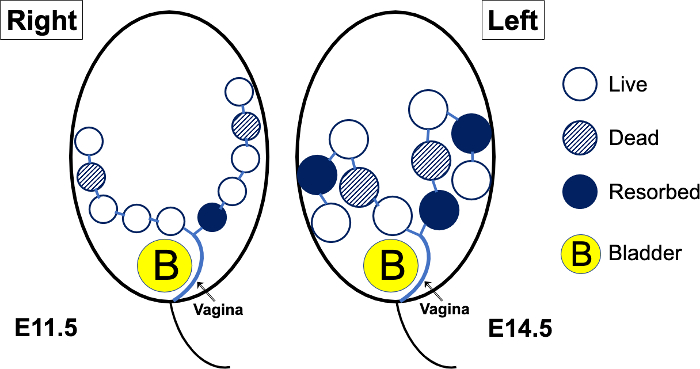
Figure 1: Schematic diagram of a theoretical pregnant mouse abdomen, imaged at E11.5, then again at E14.5. Up to mid-gestation (E10.5 or E11.5), the mouse embryos will be positioned along the right and left peripheral aspects of the abdomen. As the embryos grow, the more distal portions of the uterus and their corresponding embryos will turn outwards and posteriorly. As the embryos grow further (E15.5 and later, generally), the mouse fetuses will be positioned almost randomly in various directions, and it becomes difficult to “track” a uterus from proximal to distal. When there is prenatal lethality in a genetically engineered mouse model, the embryos (open circles) may die; the dead embryos (hatched circles) will eventually become resorbed (solid circles). Please click here to view a larger version of this figure.

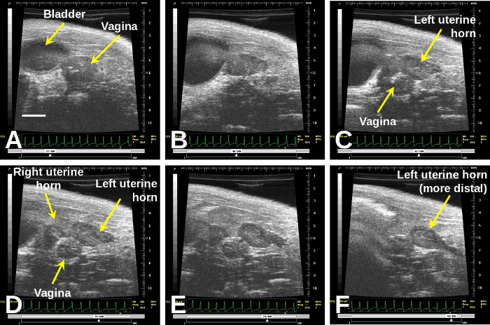
Figure 2: Once one finds the vagina (A), immediately to the right of the bladder, sweeping cranially will demonstrate the bifurcation (B) to the right and left uterine horns (D)–(F).
Scale bar (A) = 2 mm. Please click here to view a larger version of this figure.

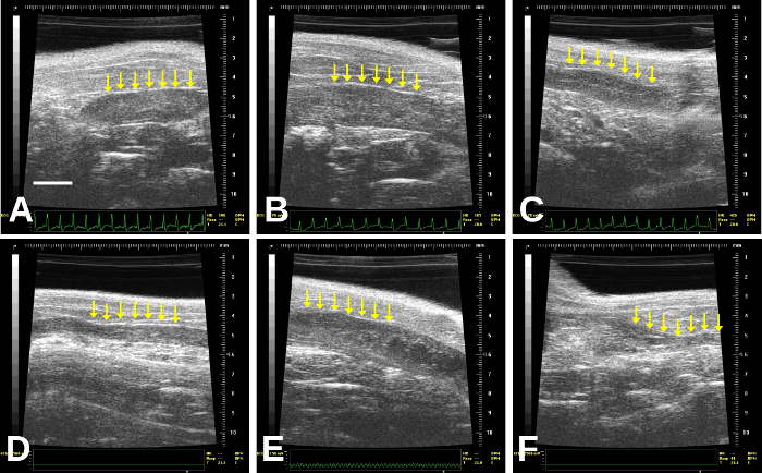
Figure 3: Images of non-gravid (non-pregnant) uterus (identified by the rows of arrows). The uterus may vary in thickness: thicker in (A), (B), (E); thin with a central thin echogenic line (C), very thin (D), or may even contain small, cystic structures that should not be mistaken for concepti (B) and (E) especially, although this may be difficult to determine. (A) is a right uterine horn; this is more difficult to follow distally in our experience due to bowel gas. (B)–(F) are left uterine horns; (F) is quite distal/lateral and so becomes more difficult to image due to increasing bowel gas artifact. Scale bar (A) = 2 mm. Please click here to view a larger version of this figure.

Figure 4: Resorbed and dead embryos have distinct appearances. Resorbed embryos, which are very commonly found, are encased within a round (gravid) uterine sac that appears relatively homogeneous except for a central echogenic (very bright) “spot”—arrows in (A) and (B). (C) shows resorbed or dead embryos; there is an entirely homogeneous, “mushy” appearance to the uterus, and we see probably 3–4 dead embryos in this frame. (D) shows a recently dead embryo, which still shows some structures; there also appears to be cellular debris in the amniotic sac. In (E), the dead embryo is much shrunken and still connected to the placenta (“P”). (F) shows a homogeneous, “mushy” appearance of an embryo that probably died 1–2 days previously, but is not yet completely resorbed. Scale bar for (A) and (D) = 2 mm. Please click here to view a larger version of this figure.

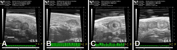
Figure 5: Early-stage embryos, from approximately E5.5 (A) and E6.5 (B) to E8.5 ((C) and (D)). There are variations in appearances, and the estimated stages here were based on timing of mating as well as the appearance of the embryos themselves. Scale bar (A) = 2 mm. Please click here to view a larger version of this figure.

Figure 6: E9.5 embryos are considerably larger than E8.5 embryos and are beginning to take form. Representative images, showing adjacent embryos, are shown in (A) and (B). Scale bars = 2 mm. Please click here to view a larger version of this figure.

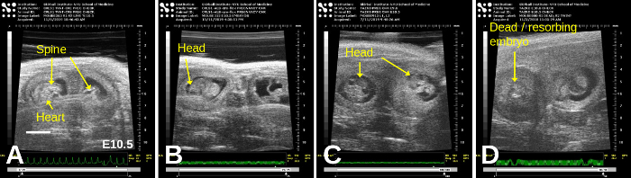
Figure 7: E10.5 embryos exhibit even clearer organs such as the head, spine, and heart. Representative images, showing adjacent embryos, are shown in all panels; in (D), a dead/resorbing embryo lies adjacent to a live embryo. Scale bar = 2 mm. Please click here to view a larger version of this figure.

Figure 8: Older embryos, approximately E12.5 (A), E14.5 (B), and E15.5 (C). Oblique planes of imaging obscure the precise anatomy somewhat, but the heart (arrow) is in the central portion of each embryo; in (C), the myocardium is now more echogenic than the blood. Please click here to view a larger version of this figure.

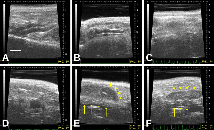
Figure 9: The bowel, which is the organ most likely to be confused with the uterus. In (E), a resorbed embryo (arrowheads) overlies a segment of bowel (arrows). In (F), a non-gravid uterus (arrowheads) overlies a short segment of bowel (arrows) Please click here to view a larger version of this figure.

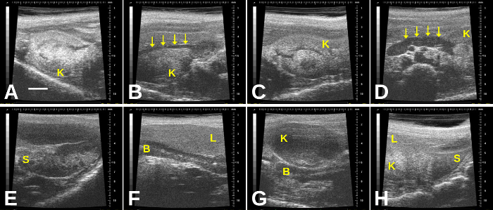
Figure 10: Additional imaging artifacts in the gravid abdomen include the kidneys, spleen, and liver. (A) Right kidney; (B) Right kidney with renal artery (arrows); (C) Left kidney; (D) Left kidney with renal artery (arrows); (E) Spleen; (F) Liver overlying a segment of bowel; (G) Kidney overlying segment of bowel; (H) Spleen, liver, and left kidney seen in one plane of imaging. B = bowel; K= kidney; L= liver; S= spleen. Scale bar (A) = 2 mm. Please click here to view a larger version of this figure.

Discussion

The most important first step in the imaging is to identify the vagina and then to determine the bifurcation of the uterine horn to the left and right. By following each uterine horn, the imager is less likely to mis-identify loops of the bowel as the uterus. Moreover, understanding the variations in the appearance of the bowel (with/without fecal matter) is important to distinguish these from the uterus; occasionally, fecal “balls” in bowel loops may mimic a gravid (pregnant) uterus. Although other authors have described the diagnosis of pregnancy and staging of mouse embryonic development^17,18,19 including the detection of resorbed embryos²⁰, this study is the first to outline the steps and potential pitfalls in imaging the gravid murine uterus.

The imager must recognize potential artifacts that may mimic an early pregnancy or gravid uterus or that may interfere with the imaging of the uterus and embryos. Following the uterine horns laterally will reduce the likelihood of mistaking other organs and artifacts in the abdomen for the uterus (and small embryos). Potential artifacts that may be mistaken for uterus, embryos, and/or obstructive items include the bowel and bowel gas, feces, spleen, liver, and stomach.

This method requires general anesthesia, and we are careful to limit: 1) time of imaging and 2) frequency of pregnancy checks, to reduce any chance of intrauterine loss due to anesthesia. Although anesthetics and analgesics appear to be safe overall during pregnancy²¹, significant exposure may have consequences on mouse embryonic growth²². As mouse knockout models often demonstrate prenatal or early perinatal death, exposure of the embryos to general anesthesia during this imaging may (at least theoretically) increase their risk of demise or influence their biology in unknown ways. While an absolute time limit is unknown, we try to limit each imaging session to no more than 15 minutes, and to 2–3 imaging sessions (maximum) per pregnancy. The “ALARA principle” is prudent here: As Low As Reasonably Achievable.

This method allows for more efficient breeding as well as rapid determination of intrauterine demise. This is especially important in experiments using knockout models that die early; other examples include toxicological studies. While a few studies have detailed the weight gain during pregnancy, it is quite clear that the weight gain early (prior to E8.5) is small and may not be different from diurnal weight changes. Furthermore, the data were derived from first-time pregnant mice only and may not reflect the confounding effects of multi-gravid mice^10,11. Timed pregnancies may not be evident early on, and especially with genetically-engineered mice, intrauterine losses may be common or even affect the entire litter. Thus, simply because a mouse does not deliver a litter does not mean she was never pregnant. Mice can be re-mated in a week if the female is not pregnant; otherwise, researchers will simply have to wait it out to see if the female has become pregnant. After skills are developed to do more than simply check for pregnancy, this method will also allow mapping and monitoring the embryos as the pregnancy progresses. In this way, the optimal timing for embryo harvest can be determined if tissues must be harvested prior to demise²³.

Materials

List of materials used in this article

Name	Company	Catalog Number	Comments
Depilatory cream
Ethanol, 70%
Fur clippers
Gauze or KimWipes
Isoflurane
Medical oxygen (optional)
Medical tape
Mouse imaging system (including anesthesia set-up and imaging platform)	Fujifilm Visual Sonics	Various	Any system with 40 MHz center-frequency ultrasound transducer probe
Razor blade (not a safety razor)
Scale (to weigh mouse)
Ultrasound gel

References

- Bogue, M. A., et al. Mouse Phenome Database: an integrative database and analysis suite for curated empirical phenotype data from laboratory mice. Nucleic Acids Research. 46, 843-850 (2018).
- Ito, R., Takahashi, T., Ito, M. Humanized mouse models: Application to human diseases. Journal of Cellular Physiology. 233 (5), 3723-3728 (2018).
- Law, M., Shaw, D. R. Mouse Genome Informatics (MGI) is the international resource for information on the laboratory mouse. Methods in Molecular Biology. 1757, 141-161 (2018).
- Rydell-Törmänen, K., Johnson, J. R. The applicability of mouse models to the study of human disease. Methods in Molecular Biology. 1940, 3-22 (2019).
- Hinton, R. B., Yutzey, K. E. Heart valve structure and function in development and disease. Annual Reviews of Physiology. 73, 29-46 (2011).
- Dickinson, M. E., et al. High-throughput discovery of novel developmental phenotypes. Nature. 537 (7621), 508-514 (2016).
- Tam, P. P. L., et al. Formation of the embryonic head in the mouse: attributes of a gene regulatory network. Current Topics in Developmental Biology. 117, 497-521 (2016).
- Palis, J. Hematopoietic stem cell-independent hematopoiesis: emergence of erythroid, megakaryocyte, and myeloid potential in the mammalian embryo. FEBS Letters. 590 (22), 3965-3974 (2016).
- Behringer, R., Gertsenstein, M., Nagy, K. V., Nagy, A. Selecting female mice in estrus and checking plugs. Cold Spring Harbor Protocols. 2016 (8), (2016).
- Heyne, G. W., et al. A simple and reliable method for early pregnancy detection in inbred mice. Journal of the American Association for Laboratory Animal Science. 54 (4), 368-371 (2015).
- Finlay, J. B., Liu, X., Ermel, R. W., Adamson, T. W. Maternal weight gain as a predictor of litter size in Swiss Webster, C57BL/6J, and BALB/cJ mice. Journal of the American Association for Laboratory Animal Science. 54 (6), 694-699 (2015).
- Zhou, Y. Q., et al. Applications for multifrequency ultrasound biomicroscopy in mice from implantation to adulthood. Physiological Genomics. 10 (2), 113-126 (2002).
- Ji, R. P., Phoon, C. K. L. Noninvasive localization of nuclear factor of activated T cells c1-/- mouse embryos by ultrasound biomicroscopy-Doppler allows genotype-phenotype correlation. Journal of the American Society of Echocardiography. 18 (12), 1415-1421 (2005).
- Kulandavelu, S., et al. Embryonic and neonatal phenotyping of genetically engineered mice. ILAR Journal. 47 (2), 103-117 (2006).
- Mu, J., Slevin, J. C., Qu, D., McCormick, S., Adamson, S. L. In vivo quantification of embryonic and placental growth during gestation in mice using micro-ultrasound. Reproductive Biology and Endocrinology. 6, 34(2008).
- Phoon, C. K. L., Turnbull, D. H. Cardiovascular imaging in mice. Current Protocols in Mouse Biology. 6 (1), 15-38 (2016).
- Phoon, C. K. L., Turnbull, D. H. Ultrasound biomicroscopy-Doppler in mouse cardiovascular development. Physiological Genomics. 14 (1), 3-15 (2003).
- Peavey, M. C., et al. A novel use of three-dimensional high-frequency ultrasonography for early pregnancy characterization in the mouse. Journal of Visualized Experiments. (128), e56207(2017).
- Greco, A., et al. High frequency ultrasound for in vivo pregnancy diagnosis and staging of placental and fetal development in mice. PLoS One. 8 (10), 77205(2013).
- Flores, L. E., Hildebrandt, T. B., Kühl, A. A., Drews, B. Early detection and staging of spontaneous embryo resorption by ultrasound biomicroscopy in murine pregnancy. Reproductive Biology and Endocrinology. 12, 38(2014).
- Norton, W. B., et al. Refinements for embryo implantation surgery in the mouse: comparison of injectable and inhalant anesthesias - tribromoethanol, ketamine and isoflurane - on pregnancy and pup survival. Laboratory Animal. 50 (5), 335-343 (2016).
- Thaete, L. G., Levin, S. I., Dudley, A. T. Impact of anaesthetics and analgesics on fetal growth in the mouse. Laboratory Animal. 47 (3), 175-183 (2013).
- Phoon, C. K. L., et al. Tafazzin knockdown in mice leads to a developmental cardiomyopathy with early diastolic dysfunction preceding myocardial noncompaction. Journal of the American Heart Association. 1 (2), (2012).
Reprints and Permissions