פרוטוקול זה מציג תהליך עבודה הניתן לשחזור עבור תחזית שימושי קרקע בריבוי תרחישים, הערכת אגירת פחמן וניתוח קשרים טופוגרפיים בנוף של אתר המורשת העולמית Yixian–Huangshan.
מאמר שיטה
תחזית שימושי קרקע תרחישית-רב ומעריך אחסון פחמן בנוף מורשת העולמית של Yixian-Huangshan
במאמר זה
סיכום
תקציר
שינויים בשימוש בקרקע משנים את אחסון הפחמן היבשתי, אך זרימות עבודה הניתנות לשחזור להערכת שינויים מבוססי תרחישים נותרות מוגבלות בנופים של אתרי מורשת עולמית המכוונים לתיירות. פרוטוקול זה משלב אוטומט תאים מסוג מרקוב מותאם אישית, חשבונאות פחמן בעלת ארבעה מאגרים השקולה למסגרת ה-Integrated Valuation of Ecosystem Services and Tradeoffs, וגלאי גיאוגרפי מבוסס פרמטרים אופטימליים כדי להעריך שינויים בשימוש בקרקע ובאחסון הפחמן ב-Yixian ובאזורים סמוכים ב-Huangshan בדרום Anhui, סין. מפות מתוך ה-China Land Cover Dataset משנים 2005, 2010 ו-2015 שימשו לכיול ולאישור מחוץ לתקופה. ארבעה תרחישים חקרים — Business As Usual, Tourism Expansion and Development, Ecological Conservation Priority, ו-Village Revitalization and Activation — סומולו עבור השנים 2030 ו-2050. אישור על פני 4,632,329 פיקסלים תקפים הניב דיוק כולל של 96.61%, מקדם Kappa של 0.850, ו-Figure of Merit של 0.107. אחסון הפחמן בבסיס היה 59.505 teragrams של פחמן, כאשר יערים תרמו 95.9%. הפסדי פחמן חזויים עד שנת 2050 נעו בין 5.01% תחת תרחיש Ecological Conservation Priority ל-13.49% תחת תרחיש Tourism Expansion and Development. הפרעות תואמות של אחד-בכל-פעם תמכו באותו דירוג של התרחישים. הגלאי הגיאוגרפי המבוסס על פרמטרים אופטימליים זיהה את השיפוע, התבליט והגובה כהקשרים הטופוגרפיים החזקים ביותר שנמדדו. הקלטים, הפרמטרים, הפלטים והסקריפטים שסופקו תומכים בשחזור התוצאות; עם זאת, יש לפרש את התרחישים כמבחני מאמץ השוואתיים ולא כתחזיות מכוילות.
מבוא
מערכות אקולוגיות יבש(יות) אוגרות פחמן בצמחייה, בקרקע ובחומר אורגני מת, ובכך תורמות לוויסות האקלים1,2. המרה של קרקעות עלולה לשנות במהירות מלאים אלה; לכן, הערכה מפורטת מרחבית היא חשובה לתכנון שימושי קרקע ולניהול פחמן.
ההיקף האנליטי בדרום Anhui כולל יערות סובטרופיים נרחבים, אגנים חקלאיים ואזורים הקשורים לאתרי המורשת העולמית של Mount Huangshan ו-Xidi–Hongcun3,4. מחקרים על כיסוי קרקע של מורשת תרבותית, תיירות באתרים המוכרזים כמורשת עולמית ושימור כפרים מסורתיים מצביעים על כך שבתנאים אלו יש צורך בשקילה משולבת של המצב האקולוגי, לחץ המבקרים וזהות המקום5,6,7.
מודלים של שימושי קרקע מבוססי תרחישים מתרגמים מעברים שנצפו להקרנות מפורטות מרחבית, וחשבונאות של מאגרי פחמן מכמתת את ההשלכות של דפוסים אלו. מחקרים קודמים שילבו סימולציית שימושי קרקע ליצירת טלאים (PLUS) או הקצאה מבוססת אוטומט תאי-מרקוב (CA–Markov) עם מסגרת הערכה משולבת של שירותי מערכת אקולוגית וטרייד-אופים (InVEST) ועם גלאי גיאוגרפי המבוסס על פרמטרים אופטימליים (OPGD) בסין ובנופים אחרים, כולל יישומים משולבים אחרונים8,9,10,11,12,13,14,15,16,17,18,19,20. מחקרים אלו מספקים תקדימים מתודולוגיים, אם כי הסימולטור המשמש כאן הוא מימוש מותאם אישית של אוטומט תאי מרקוב (Markov-CA) ולא PLUS.
מחקרים קשורים העריכו מסלולי פחמן המותנים במדיניות, מודלים משולבים של לוויינים ושימושי קרקע, אגירת פחמן רגישה לטופוגרפיה, יישומים עירוניים ובקמפוסים, ניהול פחמן בקרקע, מעברים בקרקעות חקלאיות, מיפוי יערות לאומי, ותלות בקנה מידה21,22,23,24,25,26,27,28,29,30,31,32,33,34. יחד, מחקרים אלו תומכים בהשוואה בין מספר תרחישים, תוך שהם מדגימים כי המסקנות תלויות בקנה מידה של הנתונים, במעברים בין מחלקות, בפרמטרי פחמן ובהנחות המדיניות הממודלות. היישום המותאם שנעשה בו שימוש במחקר הנוכחי מספק תהליך עבודה שקוף שבו ניתן לבחון את מטריצת המעברים, מכפילי התרחישים, הליך ההקצאה, השליפה של צפיפות הפחמן, ניתוח רגישות וניתוח קשרים טופוגרפיים בתוך מסגרת שחזור אחת. במחקר הנוכחי, הערך המעשי של תהליך העבודה המותאם הוא שמטריצת המעברים, פרמטרי התרחישים, כללי הקצאת פיקסלים, תיקוף, ניתוח רגישות, חשבונאות פחמן וניתוח קשרים טופוגרפיים מיושמים ומתועדים בתוך מסגרת חישובית ניתנת לשחזור. מבנה זה מאפשר לבחון ולשחזר את ההנחות ואת שלבי הניתוח הביניים ששימשו בניתוח התרחישים. מכיוון שתהליך העבודה לא הושווה ישירות ל-PLUS או ליישומים אחרים של CA–Markov, לא נטענת עדיפות ברמת הדיוק, היעילות או ביצועי הניבוי.
מחקרים על בקרות טופוגרפיות ואדפיות, התמדה של פחמן בקרקע גאומורפית, השפעות של קנה מידה מרחבי, יישומי OPGD, פריון ב-Huangshan, מדדי נוף, שטחים רטובים ופחמן ביערות תומכים עוד יותר בפרשנות זהירה, המבוססת על קשרים, של השפעות תבליט השטח35,36,37,38,39,40,41,42,43,44. על רקע זה, המטרה הכוללת של השיטה הנוכחית היא לספק זרימת עבודה שקופה וניתנת לשחזור עבור תחזית שימושי קרקע בריבוי תרחישים, הערכת מאגרי פחמן וניתוח קשרים טופוגרפיים בנוף מורשת העולם של Yixian–Huangshan. זרימת העבודה משתמשת במימוש מותאם של Markov-CA עם חשבונאות פחמן של ארבעה מאגרים השקולה ל-InVEST ו-OPGD, מתקפת את המודל מחוץ לתקופה עבור 2005–2015, ומבצעת ניתוח רגישות של 28 הרצות בשיטת "משתנה אחד בכל פעם" (one-at-a-time). רסטרים נלווים, כללי תרחישים, מטריצת בלבול, קובצי סביבה וסקריפטים מאפשרים בדיקה ישירה ושחזור של זרימת העבודה של הסימולציה המותאמת. זרימת העבודה מיועדת ליישומים עם רסטרים קטגוריים תואמים של כיסוי קרקע, פרמטרים של צפיפות פחמן ספציפיים למחלקה ונתונים טופוגרפיים מתאימים, כאשר המטרה היא הערכה השוואית של תרחישים ולא חיזוי מרחבי מדויק.
למחקר זה היו שלוש מטרות: (1) סימולציה של שימושי קרקע לשנים 2030 ו-2050 תחת מבחני מאמץ של "עסקים כרגיל" (BAU), הרחבה ופיתוח תיירות (TED), עדיפות לשימור אקולוגי (ECP), והחייאה והפעלת כפרים (VRA); (2) כימות מאגרי פחמן באמצעות טבלת חיפוש מלאה של תשע מחלקות וארבעה מאגרים; ו-(3) הערכת הקשרים האינדיבידואליים והמשותפים של גובה, שיפוע, כיוון צפוני ותבליט טופוגרפי עם צפיפות הפחמן בשנת 20158,9,10. מטרות אלו משלבות תחזיות שימושי קרקע, חשבונאות פחמן וניתוח קשרי תוואי השטח בתוך זרימת עבודה אחת הניתנת לשחזור, תוך שמירה על ההבחנה בין תוצאות סימולציית שימושי הקרקע לבין קשרים סטטיסטיים עם משתנים טופוגרפיים.
תוויות התרחישים מציינות הנחות השוואתיות ולא תחזיות מותאמות או תוכניות סטטוטוריות מקודדות. בהתאם לכך, השיטה מתאימה ביותר להשוואה הדירה של הנחות שימוש חלופיות בקרקע ותוצאות אחסון הפחמן הנלוות להן, ולא לפרשנות של המפות שנוצרו כתחזיות מכויילות של שימושי קרקע עתידיים.
פרוטוקול
No human participants, animals, or protected species were involved. The analysis used only publicly available remote-sensing products and published carbon-density parameters; therefore, ethics committee approval was not required.
Implement all computational procedures in Python 3.11 within an open and reproducible workflow. Follow seven sections: (1) define the study area; (2) acquire and preprocess the inputs; (3) estimate the transition matrix and initialize the custom Markov-CA; (4) configure the scenarios, sensitivity tests, and future simulations; (5) calibrate and validate the model; (6) calculate carbon storage; and (7) detect terrain associations with OPGD. Follow the complete workflow shown in Figure 1.
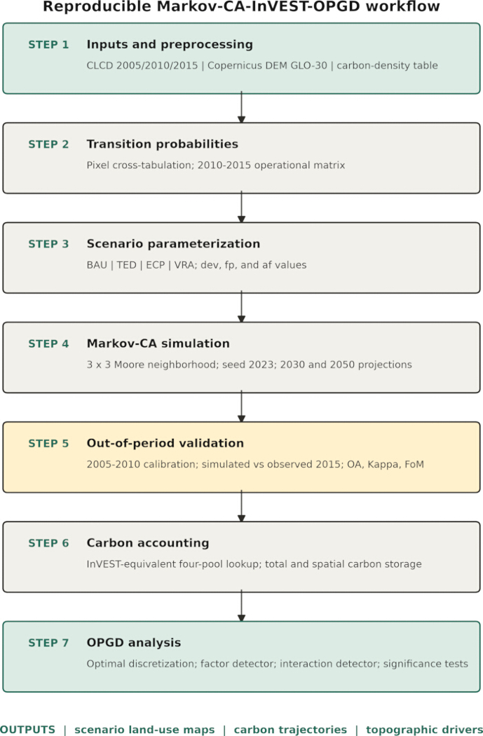
Figure 1. Reproducible workflow for multi-scenario land-use projection, carbon storage assessment, and topographic association analysis. The seven-step workflow comprises (1) input preparation and preprocessing using China Land Cover Dataset (CLCD) maps, Copernicus Digital Elevation Model (DEM) GLO-30 data, and the carbon-density table; (2) estimation of transition probabilities by pixel cross-tabulation; (3) parameterization of the Business As Usual (BAU), Tourism Expansion and Development (TED), Ecological Conservation Priority (ECP), and Village Revitalization and Activation (VRA) scenarios; (4) Markov cellular automaton (Markov-CA) simulation using a 3 × 3 Moore neighborhood; (5) out-of-period validation using overall accuracy (OA), Kappa, and Figure of Merit (FoM); (6) carbon accounting using an Integrated Valuation of Ecosystem Services and Tradeoffs (InVEST)-equivalent four-pool lookup; and (7) optimal parameters-based geographical detector (OPGD) analysis. The workflow produces scenario-specific land-use maps, carbon-storage trajectories, and assessments of topographic associations. Please click here to view a larger version of this figure.
1. Study area
- Define the analysis grid as 117.60–118.38°E and 29.72–30.22°N. Treat the Mount Huangshan and Xidi–Hongcun World Heritage properties as geographical context only; do not interpret the rectangular analytical extent or valid mask as an official administrative or World Heritage boundary3,4.
- Reproject the grid to EPSG:32650 and apply the valid mask to obtain 4,632,329 cells at 30 m resolution, representing 4,169.1 km2. Use this extent, which covers Yixian County, adjacent parts of the Huangshan Scenic Area, and northern Xiuning County, for all raster analyses (Figure 2).
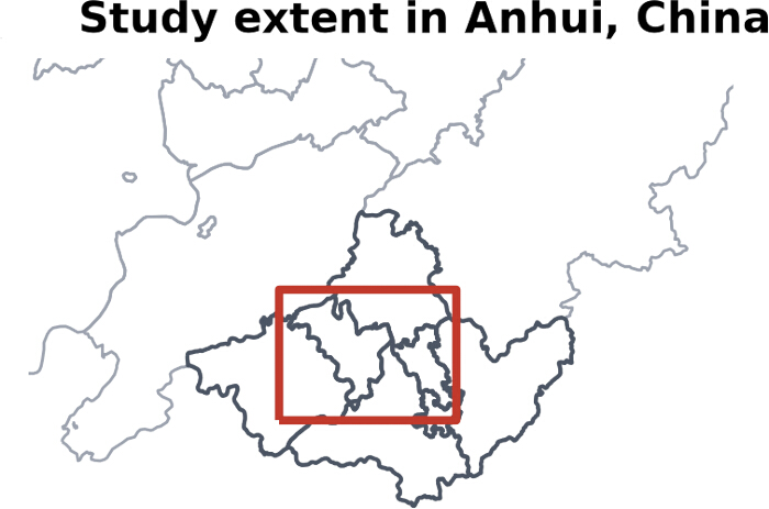
Figure 2. Study extent of the Yixian–Huangshan landscape in southern Anhui, China. Location of the analytical extent within Anhui Province, China, with the study area indicated by the red rectangle. The topographic variables used in the association analysis are presented in Figure 5. Please click here to view a larger version of this figure.
2. Data sources
- Use three input groups: CLCD annual land-cover data, Copernicus DEM GLO-30 terrain data, and a class-specific four-pool carbon-density table. Record the temporal coverage, resolution, provenance, and analytical role of each input in Table 1.
- Extract the 2005, 2010, and 2015 CLCD layers at 30 m resolution. Retain the nine classes: cropland, forest, shrub, grassland, water, snow/ice, barren, impervious, and wetland45.
- Derive elevation, slope, northness, and topographic relief from Copernicus DEM GLO-3046. Assign the complete nine-class carbon-pool values reported in Table 6 of Cheng et al.; do not apply an uncited default or zero-value convention47.
- Reproject all layers to WGS 84 / UTM zone 50N (EPSG:32650) on the common 30 m grid. Use nearest-neighbor resampling for categorical land cover and bilinear resampling for continuous terrain data.
- Apply the same valid mask to every layer before cross-tabulation, validation, carbon accounting, and OPGD sampling.
- Use Python 3.11.9 with numpy 2.4.6, scipy 1.17.1, rasterio 1.4.4, matplotlib 3.11.0, pandas 3.0.3, geopandas 1.1.4, and shapely 2.1.2. Refer to the archived environment files and relative-path scripts for exact reproduction.
- Configure the Markov-CA with a 3 × 3 Moore neighborhood and seed 2023. Initialize an independent seeded generator for each scenario-year and sensitivity run, and use seed 42 for OPGD sampling.
| Dataset | Temporal coverage | Native spatial resolution | Primary source / persistent identifier | Role in the analytical workflow |
| China Land Cover Dataset (CLCD; Yang & Huang45) | 2005, 2010, and 2015 | 30 m | Zenodo DOI: 10.5281/zenodo.4417810 | Land-use classification, change detection, validation, transition-matrix estimation, observed baseline, and Markov cellular automaton input |
| Copernicus Digital Elevation Model (DEM) GLO-30 | 2019 reference epoch; static in this study | 30 m | Copernicus Data Space Ecosystem / Microsoft Planetary Computer STAC | Elevation and derivation of slope, northness, and topographic relief using a 450 m-radius neighborhood |
| Carbon-density parameters | Static | Per land-use class; class lookup (Mg C ha⁻¹) | Cheng et al.47 Table 6 | Complete nine-class, four-pool lookup used for Integrated Valuation of Ecosystem Services and Tradeoffs-equivalent carbon accounting (Table 3) |
| Study-area analysis extent and boundary | Static | Vector / 30 m mask | Reconstructed from the manuscript extent: 117.60–118.38°E, 29.72–30.22°N; archived GeoJSON and mask | Common spatial mask, analysis extent, and analysis grid |
Table 1: Primary spatial and tabular datasets used in the analytical workflow. The table summarizes the temporal coverage, native spatial resolution, source or persistent identifier, and analytical role of the China Land Cover Dataset (CLCD), Copernicus Digital Elevation Model (DEM) GLO-30, class-specific carbon-density parameters, and study-area analysis extent. Carbon-density values are expressed in megagrams of carbon per hectare (Mg C ha−1).
3. Estimate the transition matrix and initialize the Markov-CA model
- Cross-tabulate valid CLCD pixels from 2010 to 2015. For source class i and target class j, calculate .
- Use the resulting 9 × 9 transition matrix for future scenarios. Derive a separate 2005–2010 transition matrix for model validation.
- Run the simulator as a custom Python Markov-CA implementation; do not invoke PLUS8.
- At each five-year step, take a synchronous snapshot of the starting state. Compute the transition counts from that snapshot.
- Evaluate target classes 1–9 and source classes 1–9 in ascending order. Remove each selected source pixel from further allocation so that it can transition at most once during the five-year step.
- Rank eligible candidate pixels by the start-of-step count of target-class neighbors in a 3 × 3 Moore window plus uniform random jitter from 0 to 0.5.
- Calculate the requested number of pixels for each source-to-target transition as the rounded product of the number of valid pixels in the source class, the corresponding transition probability, and the applicable scaling factor.
- Use a scaling factor of dev for transitions to impervious land and dev × fp for forest-to-impervious transitions; otherwise, use a scaling factor of 1. Cap the requested count at the number of eligible candidate pixels.
- If the requested count is smaller than the eligible candidate count, select the highest-ranked candidates based on the target-class neighborhood score plus the uniform random jitter described above; if the requested count equals the eligible candidate count, select all eligible candidates.
4. Configure scenarios, sensitivity tests, and future simulations
- Apply three parameters to the common transition matrix. Let dev scale expected transitions to impervious class 8, apply fp only to forest-to-impervious transitions, and define af as the per-step probability that cropland without an impervious Moore neighbor converts to forest.
- Set (dev, fp, af) to (1.4, 1.0, 0.005) for BAU, (6.0, 2.0, 0.001) for TED, (0.4, 0.4, 0.025) for ECP, and (2.5, 0.7, 0.012) for VRA. Use Table 2 for the corresponding computational rules, policy narratives, and parameter values.
- Interpret the multipliers as transparent low-, intermediate-, and high-development stress tests around the empirical transition matrix. Do not treat them as coefficients estimated from tourism, village-node, zoning, transport, protected-area, or ecological-redline data.
- Use the policy labels only to describe relative parameter directions. Do not interpret the labels as legal or spatial constraints encoded in the model.
- Treat dev, fp, and af as author-defined exploratory stress-test parameters rather than empirically estimated or calibrated coefficients. The nominal values specify contrasting numerical scenario assumptions for development pressure (dev), forest protection (fp), and afforestation (af); they were not fitted to observed post-2015 land-use change or interpreted as estimates of specific policy effects. Use these nominal values for the primary scenario comparisons and evaluate their robustness using the one-at-a-time sensitivity analysis described below.
- For each scenario, run the nominal 2050 case. Repeat the simulation after multiplying one of dev, fp, or af by 0.5 or 1.5 while holding the other parameters constant.
- Reinitialize seed 2023 for each of the 28 runs. Compare carbon storage, carbon loss, forest share, and impervious share, and report matched-case rankings and the full OAT ranges without treating them as probabilistic confidence intervals.
- Initialize every future simulation from observed CLCD 2015. For impervious allocation, allow cropland to remain eligible across the valid mask and require non-cropland source pixels to border start-of-step impervious cells.
- After class-to-class allocation, convert qualifying cropland to forest independently with probability af. Run three five-year steps for the 2030 projection and seven five-year steps for the 2050 projection.
- Preserve class 0 outside the valid mask. Export every projected map at 30 m resolution.
| Scenario | Implemented computational rule | Policy narrative (not an encoded constraint) | Parameters (dev / fp / af) |
| Business As Usual (BAU) | Moderate impervious multiplier; baseline forest susceptibility; 0.5% isolated-cropland afforestation per step | Continuation benchmark | 1.4 / 1.0 / 0.005 |
| Tourism Expansion and Development (TED) | Strong impervious multiplier; doubled forest-to-impervious susceptibility; weak afforestation | High-development stress test | 6.0 / 2.0 / 0.001 |
| Ecological Conservation Priority (ECP) | Reduced impervious conversion and forest susceptibility; strongest afforestation | Ecological-conservation stress test | 0.4 / 0.4 / 0.025 |
| Village Revitalization and Activation (VRA) | Intermediate impervious multiplier; forest susceptibility below BAU; intermediate afforestation | Village-revitalization narrative; no village-node layer | 2.5 / 0.7 / 0.012 |
Table 2: Computational rules and parameter values for the four land-use scenarios. The table summarizes the implemented computational rules, policy narratives, and parameter values for the Business As Usual (BAU), Tourism Expansion and Development (TED), Ecological Conservation Priority (ECP), and Village Revitalization and Activation (VRA) scenarios. Policy narratives describe the intended interpretation of each scenario and are not encoded spatial constraints. dev, impervious-development multiplier; fp, forest-to-impervious susceptibility multiplier; af, isolated-cropland afforestation fraction per simulation step.
5. Calibrate and validate the land-use model
- Estimate the calibration matrix from observed 2005–2010 change. Simulate 2015 from observed 2010 using seed 2023.
- Compare the simulated 2015 map pixel by pixel with observed CLCD 2015 within the valid mask. Calculate overall accuracy, Kappa, the 9 × 9 confusion matrix, and FoM for changed cells48.
- Exclude invalid cells from both the numerator and denominator of the validation calculations to prevent outside-mask zeros from inflating agreement.
- Interpret overall accuracy and Kappa jointly with FoM because stable forest and cropland dominate the former metrics, whereas FoM evaluates the smaller changed-cell set. Use the validation results to support regional scenario comparison; do not interpret them as establishing precise change-location forecasting.
6. Calculate carbon storage
- For each valid pixel, assign the four class-specific carbon-pool densities listed in Table 3. Sum the four pool densities to obtain the total carbon density in Mg C ha⁻1.
- Multiply the total carbon density by the 0.09 ha pixel area. Convert the resulting Mg C values to Tg C.
- Apply this lookup calculation as the algebraic equivalent of the InVEST Carbon Storage formulation. Do not apply a sequestration-rate, valuation, or economic module9,47.
| Land-use class (CLCD) | Aboveground C (Mg C ha⁻¹) | Belowground C (Mg C ha⁻¹) | Soil C (Mg C ha⁻¹) | Dead organic C (Mg C ha⁻¹) | Total C (Mg C ha⁻¹) | Source |
| 1 Cropland | 3.56 | 7.45 | 26.9 | 9.82 | 47.73 | Cheng et al.47, Table 6 |
| 2 Forest | 53.59 | 17.36 | 84.85 | 2.8 | 158.6 | |
| 3 Shrub | 4.25 | 4.65 | 72.9 | 1.59 | 83.39 | |
| 4 Grassland | 4.15 | 16.58 | 78.2 | 1.55 | 100.48 | |
| 5 Water | 6.38 | 0 | 0 | 0.12 | 6.5 | |
| 6 Snow/ice | 0 | 0.33 | 5.35 | 0 | 5.68 | |
| 7 Barren | 1.3 | 0.33 | 21.6 | 0 | 23.23 | |
| 8 Impervious | 0 | 0 | 9.28 | 0 | 9.28 | |
| 9 Wetland | 12.24 | 9.18 | 95.73 | 4.08 | 121.23 |
Table 3: Carbon-density parameters for the nine China Land Cover Dataset land-use classes used in carbon accounting. Aboveground, belowground, soil, dead organic, and total carbon-density values are provided for each China Land Cover Dataset (CLCD) land-use class. Total carbon density represents the sum of the four carbon pools. All carbon-density values are expressed in megagrams of carbon per hectare (Mg C ha−1). Values were obtained from Cheng et al.47, Table 6.
7. Detect topographic associations with OPGD
- Use 2015 carbon density as the response variable and elevation, slope, northness, and topographic relief as the explanatory factors. Sample 200,000 valid pixels using seed 42.
- For each explanatory factor, test 2–15 quantile intervals. Retain the discretization that produces the maximum q-value.
- Calculate analytic F-test p-values and permutation p-values using 999 permutations. Calculate the permutation p-value as p = (exceedances + 1) / 1000.
- Combine the optimized strata for each pair of explanatory factors to calculate the interaction results. Interpret all factor and interaction outputs as spatial associations rather than causal effects10.
תוצאות
התבצעות מרחבית ודינמיקה זמנית של שימושי קרקע
תהליך העבודה האנליטי, היקף המחקר ומערכי הנתונים הראשוניים מסוכמים ב- איור 1, איור 2ו- טבלה 1בהתאמה. איור 1 מציג את תזרים העבודה בן שבעת השלבים המשמש להשלכת שימושי קרקע, תיקוף, חשבונאות פחמן וניתוח קשרים טופוגרפיים. איור 2 מציג את המיקום ואת ההיקף האנליטי של אזור המחקר. טבלה 1 מסכם את הכיסוי הזמני, הרזולוציה המרחבית, המקור והתפקיד האנליטי של מערכי הנתונים המרחביים והטבלאיים העיקריים. השוואה בין נתוני סימולציה לשנת 2015 לבין נתוני תצפית של CLCD 2015 על פני 4,632,329 פיקסלים תקפים הניבה OA = 96.61%, Kappa = 0.850, ו-FoM = 0.107. ההסכמה נשלטה על ידי יערות ואדמות חקלאיות יציבות, בעוד שערך ה-FoM, המתמקד בשינויים, הצביע על דיוק מוגבל בשחזור מיקומי השינוי. לפיכך, התיקוף תומך בניתוח תסריטים השוואתיים ולא בחיזוי מרחבי מדויק. טבלה נלווית 1 (גיליון S3)מספק את מדדי התיקוף, את מספר הפגיעות (hits), הפספוסים (misses), ההתרעות השגויות (false alarms) ומטריצת בלבול (confusion matrix) מלאה. הארכיון מכיל את רסטר התיקוף ואת הסקריפט המדויק ששימש לחישוב.
במהלך 28 הרצות הרגישות, כל הפרעה תואמת שימרה את הדירוג ECP > BAU > VRA > TED. טווחים של אובדן פחמן היו 4.22–5.86% עבור ECP, 6.87–8.55% עבור BAU, 6.99–9.61% עבור VRA, ו-10.45–15.84% עבור TED. הטווחים של BAU ו-VRA חופפים; לכן, הפרשנות מוגבלת לסדר של מקרים תואמים ולא להפרדה מלאה של טווחי ה-OAT. תוצאות רגישות מלאות מובאות ב-Supplementary Table 1 (worksheet S4) וב-Supplementary Figure 1. מטריצת התפעול לשנים 2010–2015, המובאת ב-Supplementary Table 1 (worksheet S1), הראתה הסתברויות שימור של 98.23% עבור יער, 94.66% עבור קרקע חקלאית, ו-99.43% עבור קרקע בלתי חדירה. המעברים הגדולים ביותר מחוץ לאלכסון היו מקרקע חקלאית לקרקע בלתי חדירה (3.39%), מקרקע חקלאית ליער (1.71%), ומייער לקרקע חקלאית (1.71%). במהלך אותה תקופה, כיסוי היער פחת מ-87.63% ל-86.27%, בעוד ששטח הקרקע החקלאית עלה מ-10.99% ל-11.92% וקרקע בלתי חדירה עלתה מ-1.08% ל-1.50%. Figure 3A,B מציגים את דפוסי שימוש הקרקע שנצפו בשנים 2010 ו-2015, בהתאמה, ו-Figure 4 מציג את מחלקות השינוי התואמות ללא הסקת גורמים שלא נכללו בניתוח.
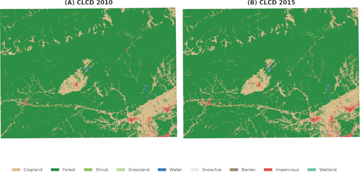
איור 3. דפוסי שימושי קרקע שנצפו בנוף Yixian–Huangshan בשנים 2010 ו-2015. מפות ממאגר נתוני כיסוי הקרקע של סין (CLCD) המציגות את ההתפלגות המרחבית של תשע מחלקות שימושי קרקע בתוך היקף הניתוח. (A) שימושי קרקע שנצפו בשנת 2010. (B) שימושי קרקע שנצפו בשנת 2015. מחלקות שימושי הקרקע כוללות שטחים חקלאיים, יער, שיחים, שטחים דשאיים, מים, שלג/קרח, קרקע צחיחה, משטחים בלתי חדירים וביצות. אנא לחץ כאן כדי לצפות בגרסה גדולה יותר של איור זה.
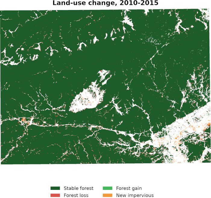
איור 4שינוי בשימוש בקרקע שנצפה בנוף של Yixian–Huangshan בין השנים 2010 ל-2015. המפה מציגה את ההתפלגות המרחבית של יער יציב, אובדן יער, תוספת יער ומשטחים בלתי חדירים שפותחו לאחרונה בין מפות מערך נתוני כיסוי הקרקע של סין משנת 2010 ושנת 2015. אזורים לבנים מייצגים מיקומים שלא סווגו לארבע קטגוריות שינוי מוצגות אלו. אנא לחצו כאן כדי לצפות בגרסה מורחבת של איור זה.
מאפייני השטח והטרוגניות טופוגרפית
בתוך המסכה התקפה, הגובה נע בין 82.3 ל-1,830.3 m (ממוצע, 388.0 m), השיפוע בין 0 ל-87.3° (ממוצע, 22.4°), החשיפה לצפון (northness) בין −1 ל-1, והבליטה הטופוגרפית בין 3.2 ל-1,398.2 m (ממוצע, 230.0 m). הבליטה הוגדרה כטווח הגבהים המקומי בתוך שכונה מעגלית ברדיוס של 450 m, אשר יושמה באמצעות טביעת רגל של 31 × 31 פיקסלים. איור 5A–D מציג את הגובה, השיפוע, החשיפה לצפון והבליטה הטופוגרפית, בהתאמה. שכבות אלו מאפיינות וריאציה מרחבית של תוואי השטח; כל מנגנון אקולוגי תואם נחשב כהיפותזה ולא כתוצאה סיבתית35,36,37,38,39,40,41,42,43,44.

איור 5. משתנים טופוגרפיים ששימשו בניתוח המתאם. התפלגויות מרחביות של ארבעת המשתנים הטופוגרפיים לאורך היקף הניתוח: (A) גובה, מבוטא במטרים; (B) שיפוע, מבוטא במעלות; (C) כיוון צפון (northness), מבוטא בסולם מ-1- עד 1; ו-(D) תבליט טופוגרפי, מבוטא במטרים. משתנים אלו שימשו בניתוח גלאי גאוגרפי מבוסס פרמטרים אופטימליים של המתאמים האינדיבידואליים והמשותפים שלהם עם צפיפות הפחמן בשנת 2015. אנא לחצו כאן כדי לצפות בגרסה גדולה יותר של איור זה.
תחזיות שימוש בקרקע בריבוי תרחישים
מטריצת המעבר המשותפת ופרמטרי התרחישים המסוכמים בTable 2 הניבו מסלולי צבירה מובחנים תוך שימוש במזהי מחלקות כיסוי הקרקע המספריים המופיעים בSupplementary Table 2. Figure 6 מציג את החלקים הנצפים והחזויים של יערות, שטחי גידולים חקלאיים ומשטחים בלתי חדירים, בעוד שFigure 7A–D מציג את התחזיות המרחביות עבור BAU, TED, ECP ו-VRA לשנת 2030, בהתאמה, וFigure 7E–H מציג את התחזיות התואמות לשנת 2050. עד שנת 2050, כיסוי היערות חזה להוות 78.0% תחת BAU, 74.6% תחת TED, 80.3% תחת ECP ו-78.2% תחת VRA; החלקים התואמים של משטחים בלתי חדירים היו 6.3%, 17.6%, 2.8% ו-9.0%. ביחס לנתונים שנצפו ב-2015, ההתרחבות החזויה של משטחים בלתי חדירים הייתה בערך 202 km2 תחת BAU, 675 km2 תחת TED, 57 km2 תחת ECP ו-317 km2 תחת VRA. ערכים אלו הם פלטי מבחני מאמץ ולא תחזיות מותאמות. השינויים החזויים מקובצים מרחבית מכיוון שדירוג המועמדים משתמש בספירות שכנות של מחלקת היעד, והמרה של קרקע שאינה חקלאית למשטחים בלתי חדירים מוגבלת לתאי קצה. המודל אינו כולל שכבות של מסדרונות תחבורה, צמתי כפרים, אזורי הגנה, קווים אדומים אקולוגיים או תכנון סטטוטורי; לכן, התאמה נראית לתשתיות ספציפיות או לאזורים מוסדרים אינה מייצגת אפקט מקודד.
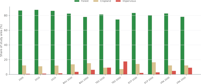
איור 6. נתחים נצפים וחזויים של מחלקות שימושי קרקע עיקריות תחת ארבעה תרחישים. מוצג אחוז שטח המחקר occupied ביערות, שטחי חקלאות ומשטחים בלתי חדירים עבור השנים הנצפות 2005, 2010 ו-2015, ועבור תחזיות לשנים 2030 ו-2050 תחת התרחישים: Business As Usual (BAU), Tourism Expansion and Development (TED), Ecological Conservation Priority (ECP), ו-Village Revitalization and Activation (VRA). העמודות מייצגות את הנתח המודל מתוך סך שטח המחקר עבור כל מחלקת שימוש בקרקע; פסי שגיאה אינם רלוונטיים מכיוון שהערכים הם תוצרי תרחישים דטרמיניסטיים ולא הערכות מבוססות חזרות. אנא לחצו כאן כדי לצפות בגרסה גדולה יותר של איור זה.
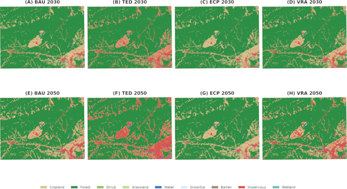
איור 7. התפלגות מרחבית חזויה של שימושי קרקע תחת ארבעה תרחישים בשנים 2030 ו-2050. דפוסי שימושי קרקע חזויים תחת התרחישים: עסקים כרגיל (BAU), הרחבה ופיתוח תיירות (TED), עדיפות לשימור אקולוגי (ECP), והחייאה והפעלה של כפרים (VRA). (A–D) תחזיות עבור BAU, TED, ECP ו-VRA, בהתאמה, לשנת 2030. (E–H) תחזיות עבור BAU, TED, ECP ו-VRA, בהתאמה, לשנת 2050. סוגי שימושי הקרקע כוללים אדמה חקלאית, יער, שיחים, שטחי עשב, מים, שלג/קרח, קרקע עירו, משטחים בלתי ח проחמימים וביצות. כל סימולציות התרחישים אותחלו ממפת ה-CLCD שנצפתה בשנת 2015; לפיכך, תאים ללא מעבר חזוי בשימושי הקרקע שומרים על סוג שימושי הקרקע ועל הדפוס המרחבי הבסיסי משנת 2015. אנא לחץ כאן כדי לצפות בגרסה גדולה יותר של איור זה.
דינמיקת אגירת פחמן תחת תחזיות של תרחישים מרובים
יישום טבלת ההתייחסות המלאה לארבעה מאגרים בTable 3 הניב 59.505 Tg C לשנת 2015, שווה ערך לצפיפות ממוצעת של 142.73 Mg C ha−1. יערות היוו 57.04 Tg C (95.9%), בעוד ששטחי חקלאות היוו 2.37 Tg C (4.0%). קרקע בלתי חדירה תרמה תרומה קטנה אך שאינה אפס, מכיוון שהמקור שאומץ מייחס למחלקה זו 9.28 Mg C ha−1. בתוך מחלקת היערות, מאגרי הקרקע, מעל פני השטח, מתחת לפני השטח והחומר האורגני המת, ייצגו 53.5%, 33.8%, 10.9% ו-1.8% מסך הפחמן, בהתאמה31,32,33,34,44,47. כל התרחישים הניבו אגירת פחמן נמוכה יותר בשנת 2050 מאשר בשנת 2015. האגירה החזויה הייתה 54.895 Tg C תחת BAU (הפסד של 7.75%), 51.475 Tg C תחת TED (13.49%), 56.523 Tg C תחת ECP (5.01%), ו-54.540 Tg C תחת VRA (8.34%). ההפרש בין ECP ל-TED היה 5.048 Tg C. ניגודים אלו נובעים מהפרמטרים המספריים שהוטלו ואינם מעריכים את ההשפעות של מדיניות ספציפית. Figure 8A מציג את סך אגירת הפחמן בשנת 2015 ואת תחזיות התרחישים לשנים 2030 ו-2050; Figure 8B מציג את צפיפויות הפחמן הממוצעות התואמות; Figure 8C מציג את אובדן הפחמן עד שנת 2050 ביחס לקו הבסיס של 2015; ו-Figure 8D מראה את הקשר בין נתח היער החזוי לבין אובדן הפחמן. הערכים הם פלטי תרחישים דטרמיניסטיים ולא הערכות המבוססות על חזרות.
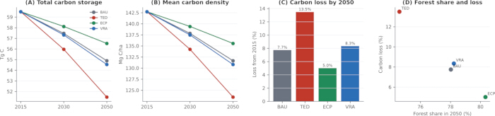
איור 8. אחסון פחמן חזוי והקשר שלו עם כיסוי היער תחת ארבעה תרחישי שימוש בקרקע. (A) סך אחסון הפחמן בשנת 2015 והתחזית לשנים 2030 ו-2050 תחת התרחישים: המשך המגמה הקיימת (BAU), הרחבה ופיתוח תיירות (TED), עדיפות לשימור אקולוגי (ECP), והחייאה והפעלה של כפרים (VRA), מבוטא בטראגרמים של פחמן (Tg C). (B) צפיפות פחמן ממוצעת עבור השנים והתרחישים המתאימים, מבוטאת במגהגרמים של פחמן לדונם (Mg C ha-1). (C) אחוז האובדן בסך אחסון הפחמן עד שנת 2050 ביחס לקו הבסיס של 2015 עבור כל תרחיש. (D) הקשר בין נתח היער החזוי של אזור המחקר בשנת 2050 לבין אחוז אובדן הפחמן ביחס לשנת 2015 עבור כל תרחיש. הערכים הם פלטי תרחישים דטרמיניסטיים; פסי שגיאה אינם רלוונטיים. אנא לחצו כאן כדי לצפות בגרסה גדולה יותר של איור זה.
קשרים טופוגרפיים עם ההטרוגניות המרחבית של אגירת פחמן
גלאי גורמי ה-OPGD דירג את השיפוע (slope) במקום הראשון (q = 0.557), ואחריו את התבליט הטופוגרפי (topographic relief) (q = 0.460), הגובה (elevation) (q = 0.352), והכיוון לצפון (northness) (q = 0.003), כפי שמוצג ב-איור 9A. ב-999 פרמוטציות, ערך ה-p של הפרמוטציה עבור כל גורם היה 0.001, הערך המינימלי שניתן להשיג; ערכי ה-p של מבחן F אנליטי היו גם הם נמוכים מ-0.001. הסטטיסטיקות המלאות של גלאי הגורמים והאינטראקציות, כולל מרווחי דיסקרטיזציה אופטימליים וערכי p אנליטיים ושל פרמוטציות, מופיעות ב-טבלה נלווית 3. יש להבחין בין מובהקות סטטיסטית לבין גודל האפקט: הקשר עם הכיוון לצפון היה זניח במונחים מעשיים, וכל ערכי ה-q מייצגים קשרים בתוך ארבעת משתני השטח שנבחנו ולא השפעות סיבתיות10,40. כל זוגות הגורמים הניבו ערכי q של אינטראקציה הגבוהים יותר מהערך הגבוה מבין ערכי ה-q האינדיבידואליים שלהם. האינטראקציות החזקות ביותר היו שיפוע ∩ תבליט (q = 0.628), גובה ∩ שיפוע (q = 0.618), וגובה ∩ תבליט (q = 0.510), כפי שמוצג ב-איור 9B. ערכים אלו מעידים על קשרים מרובדים (stratified associations) חזקים יותר עבור גורמים מזווגים, אך אינם מבססים מנגנון גאומורפולוגי כיוון שקרקע, אקלים, גיל היער, ניהול ונגישות לא נכללו במודל.
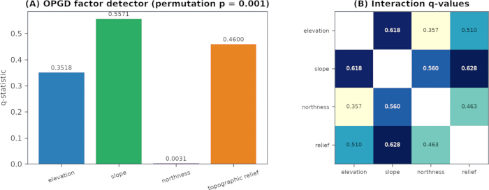
איור 9. קשרי טופוגרפיה עם צפיפות הפחמן בשנת 2015 שזוהו באמצעות הגלאי הגיאוגרפי המבוסס על פרמטרים אופטימליים. (A) סטטיסטיקות q של גלאי-גורמים (Factor-detector) עבור גובה, שיפוע, צפוניות ותבליט טופוגרפי. ערכי ה-q בהתאמה הם 0.3518, 0.5571, 0.0031 ו-0.4600; מבחני פרמוטציה הניבו p = 0.001. (B) ערכי q של גלאי-אינטראקציה (Interaction-detector) עבור שילובים זוגיים של ארבעת המשתנים הטופוגרפיים. ערכי q גבוהים יותר מעידים על קשרים סטטיסטיים חזקים יותר עם ההתפלגות המרחבית של צפיפות הפחמן בשנת 2015. OPGD, גלאי גיאוגרפי מבוסס פרמטרים אופטימליים. אנא לחצו כאן כדי לצפות בגרסה גדולה יותר של איור זה.
תוצאות כלליות
איור 10A–D מסכם את התוצאים העיקריים של תהליך העבודה: נתח היער החזוי, סך אחסון הפחמן, דירוג הקשרים הטופוגרפיים והמדדים הכמותיים המרכזיים, בהתאמה. קו הבסיס האנליטי לשנת 2015 הכיל 59.505 Tg C. בארבעה סטים של פרמטרים גששיונים, ההפסדים החזויים עד שנת 2050 נעים בין 5.01% ל-13.49%, וכל מקרי הרגישות התואמים שימרו את הדירוג ECP > BAU > VRA > TED. שיפוע ותבליט הראו את קשרי השטח החזקים ביותר שנבחנו. בהינתן FoM = 0.107 והשמטת שכבות תכנוניות, סוציו-אקונומיות ואקלימיות מפורשות, התוצאות תומכות בהערכה אזורית השוואתית ולא בחיזוי מרחבי דטרמיניסטי.
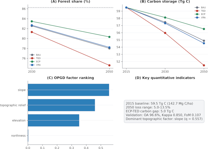
איור 10. סיכום של תוצאי שימושי קרקע ואגירת פחמן חזויות וקשרי טופוגרפיה. (A) חלק היער החזוי מאזור המחקר בשנת 2030 ובשנת 2050 תחת תרחישי "עסקים כרגיל" (BAU), הרחבה ופיתוח תיירות (TED), עדיפות לשימור אקולוגי (ECP), והחייאה והפעלה של כפרים (VRA); הקו המקווקו מציין את חלק היער בנקודת הייחוס של 2015. (B) סך אגירת הפחמן בשנת 2015 והתחזית לשנים 2030 ו-2050 תחת ארבעת התרחישים, מבוטא בטרגרמים של פחמן (Tg C). (C) דירוג של גובה, שיפוע, צפוניות ותבליט טופוגרפי בהתאם לסטטיסטיקת q שהתקבלה באמצעות גלאי גיאוגרפי מבוסס פרמטרים אופטימליים (OPGD), כאשר ערכי q גבוהים יותר מעידים על קשרים סטטיסטיים חזקים יותר עם צפיפות הפחמן בשנת 2015. (D) סיכום של מדדי כמות מרכזיים, הכוללים אגירה וצפיפות פחמן בנקודת הייחוס, טווח אובדן הפחמן החזוי ל-2050, ההבדל באגירת הפחמן בין תרחישי ECP ו-TED, מדדי תיקוף, והקשר הטופוגרפי החזק ביותר שנבחן. OA, דיוק כולל; FoM, מדד איכות (Figure of Merit); Mg C ha-1, מגהגרמים של פחמן לדונם. אנא לחץ כאן כדי להציג גרסה גדולה יותר של איור זה.
איור משלים 1. ניתוח רגישות של פרמטר אחד בכל פעם (One-at-a-time) לאחסון פחמן בשנת 2050 תחת ארבעת תרחישי שימוש הקרקע. (A) אחסון פחמן נומינלי בשנת 2050 וטווח הרגישות המלא של OAT עבור BAU, TED, ECP ו-VRA. נקודות מציינות את ערכי התרחיש הנומינליים, וטווחים אנכיים מציינים את ערכי אחסון הפחמן המינימליים והמקסימליים שהתקבלו על ידי הכפלת אחד מהפרמטרים dev, fp, או af ב-0.5 או 1.5 תוך שמירה על הפרמטרים האחרים קבועים. (B) שינוי באחסון הפחמן בשנת 2050 ביחס לערך התרחיש הנומינלי התואם בעקבות הפרעות של 0.5× ו-1.5× ל-dev, fp, ו-af. ערכים מעל אפס מצביעים על אחסון פחמן גדול יותר מהמקרה הנומינלי, וערכים מתחת לאפס מצביעים על אחסון פחמן נמוך יותר. הטווחים מייצגים הפרעות דטרמיניסטיות של פרמטר אחד בכל פעם ואינם רווחי סמך הסתברותיים.אנא לחצו כאן כדי להוריד קובץ זה.
טבלה נלווית 1. מטריצת מעברי שימושי קרקע, פרמטריזציית תרחישים, תיקוף המודל ותוצאות ניתוח רגישות של פרמטר אחד בכל פעם (one-at-a-time). חוברת העבודה כוללת ארבעה גיליונות: S1, מטריצת מעברי שימושי קרקע תפעולית לשנים 2010–2015; S2, ערכי פרמטרים, כללים שיושמו וגבולות פרשנות עבור ארבעת התרחישים; S3, מטריצת בלבול (confusion matrix) של 9 × 9 ותוצאות תיקוף המודל הנלוות; ו-S4, תוצאות רגישות נומינליות ושל פרמטר אחד בכל פעם, שהתקבלו על ידי שינוי של dev, fp ו-af ב-0.5× ו-1.5× תוך השארת הפרמטרים האחרים קבועים. טווחי הרגישות מייצגים הפרעות פרמטריות דטרמיניסטיות ואינם רווחי סמך הסתברותיים.אנא לחצו כאן להורדת קובץ זה.
טבלה נלווית 2. מזהי סוגי כיסוי קרקע ששימשו בזרימת העבודה החישובית. הטבלה מפרטת את המזהים המספריים של הסוגים ואת סוגי כיסוי הקרקע התואמים להם ששימשו בניתוחי הראסטר. סוג 0 מציין NoData מחוץ למסכת אזור המחקר התקפה; סוגים 1–9 מציינים שטח חקלאי, יער, שיחים, שטח עשב, מים, שלג/קרח, שטח צחיח, משטח בלתי חדיר וביצה, בהתאמה.אנא לחצו כאן להורדת קובץ זה.
טבלה משלימה 3. תוצאות גלאי גורמים ואינטראקציות OPGD עבור צפיפות פחמן בשנת 2015. הטבלה מציגה סטטיסטיקות q אופטימליות, מספר an-discretization intervals, ערכי p של מבחן F אנליטי, וערכי p של פרמוטציה המבוססים על 999 פרמוטציות עבור גובה, שיפוע, צפוניות ותבליט טופוגרפי. תוצאות אינטראקציות זוגיות מציגות את סטטיסטיקת ה- q של האינטראקציה, סטטיסטיקות q של גורמים בודדים וסיווג האינטראקציה. הסטטיסטיקות המדווחות מייצגות קשרים מרחביים ואינן קובעות השפעות סיבתיות.אנא לחצו כאן להורדת קובץ זה.
הערה נלווית 1. תיאורים של כל פאנל, מקורות נתונים והערות פרשנות עבור איורי כתב היד. הערה זו מזהה את התוכן ואת מקור הנתונים הבסיסי עבור פאנלים בודדים באיורים, ומספקת מידע בנוגע להיקפים מרחביים משותפים, מידע כפול ופרשנות של המשתנים המוצגים.אנא לחצו כאן להורדת קובץ זה.
ארכיון נתונים משלימים (דחוס). הארכיון מכיל 26 קבצי GeoTIFF מוכנים לניתוח, קבצי גבולות, מטא-נתונים, תוצאות, סקריפטים, איורים, חוברות עבודה, קבצי סביבת חישוב מדויקים, קובץ README וסכומי ביקורת SHA-256.
דיון
בארבעת מבחני המאמץ, אחסון הפחמן פחת ככל שהמעברים המדומים שינו את הפרופורציות של מחלקות כיסוי קרקע בעלות צפיפות גבוהה ונמוכה יותר. TED הניב את הירידה הגדולה ביותר, בעוד ש-ECP הניב את הקטנה ביותר. שלב קריטי ביישום הפרוטוקול הוא לפיכך הגדרתם ופירושם של הפרמטרים dev, fp ו-af. מכיוון שההבדלים בין התרחישים נובעים מערכים מוטלים אלו, הם מייצגים תגובות מודל מותנות ולא השפעות נצפות של פיתוח תיירות, התחדשות כפרית או רגולציה אקולוגית. עד שנת 2050, אחסון הפחמן החזוי תחת TED היה נמוך ב-5.048 Tg C מאשר תחת ECP. תחת טבלת ההתייחסות (lookup) המאומצת, המרת הקטר אחד של יער לקרקע בלתי חדירה מפחיתה את המלאי המוקצה ב-149.32 Mg C, בעוד שהמרה מאדמה חקלאית לקרקע בלתי חדירה מפחיתה אותו ב-38.45 Mg C. ניגודי חשבונאות אלו מסבירים את ההשפעה החזקה של המרת יערות מדומה על האחסון הכולל. עם זאת, הסתמכות על ערכים השגורים בספרות ללא כיול מקומי מכניסה אי-ודאות להערכות המוחלטות.
שלב קריטי נוסף הוא הגזירה והדיסקרטיזציה של משתני השטח ששימשו ב-OPGD. תבליט טופוגרפי נמצא קשור לצפיפות פחמן לאחר דיסקרטיזציה אופטימלית (q = 0.460). התבליט הוגדר כטווח הגבהים המקומי בתוך שכנות מעגלית ברדיוס של 450 m, שיושמה באמצעות טביעת רגל של 31 × 31 פיקסלים. תאים בעלי תבליט גבוה עשויים לחפוף לשטח מיוער ותלול, אך OPGD אינו יכול להבחין בין שטח, נגישות, היסטוריית שימושי קרקע, קרקע, ניהול והסברים מתואמים אחרים. שכבות שטח מזווגות הניבו ערכי q גבוהים יותר מאשר גורמים בודדים, במיוחד עבור שיפוע ∩ תבליט (q = 0.628). תבנית זו היא תיאורית ולא מכניסטית. באופן דומה, ערך ה-<q> הנמוך עבור כיוון צפוני (0.003) אינו מוכיח כי הניגודים בקרינת השמש חלשים; בדיקת הסבר זה דורשת מדידות של קרינה, מיקרו-אקלים, צמחייה ומדידות שדה.
השיטה תומכת ביצירת היפותזות אזוריות: הגבלה של המרת יערות מדומה, מיתון של התרחבות שטחים בלתי חדירים, והגברת המעבר משטחי גידול ליערות משמרים יותר פחמן שהוקצה. מרשמים ספציפיים לאתרים דורשים ראיות נוספות. לצורך התאמת תהליך העבודה ליישומים ממוקדי-החלטה, יש לשלב שכבות מאושרות של אזורים מוגנים, קווי אדום אקולוגיים, תחבורה, חלקות קרקע וצמתי כפרים, יחד עם הערכות של השתתפות בעלי עניין, פשרות בשירותי מערכת אקולוגית, תמריצים, עלויות שיקום, שירותים תרבותיים, פרנסה ומגוון ביולוגי49,50,51,52,53,54,55,56. הרחבות אלו חשובות כיוון שהפרוטוקול הנוכחי אינו מקודד אילוצים מרחביים או סוציו-אקונומיים כאלו. הספרות הרחבה יותר מצביעה גם על כך שאסטרטגיות אחסון צמחים, מבנה היער, צמחייה שאינה עץ, התנהגות תיירותית והשפעות מחזור החיים של הסביבה הבנויה דורשות ניתוחים הנבדלים מחישוב כיסוי הקרקע הנוכחי57,58,59,60,61.
מספר מגבלות מגדירות את השימוש והפירוש המתאימים של השיטה. אלו כוללות צפיפויות פחמן המבוססות על ספרות ללא כיול שטח מקומי, שגיאת סיווג CLCD פוטנציאלית, מודל Markov-CA מותאם ופשוט, מדד ביצועים (FoM) לתיקוף הממוקד בשינוי של 0.107, פרמטרים של מבחן מאמץ שאינם מותאמים (non-fitted), והערכה סטוכסטית המבוססת על גרעין (seed) בודד. מגבלות נוספות הן תכנון של גורם אחד בכל פעם (one-factor-at-a-time) במקום ניתוח אי-ודאות הסתברותי, השמטת שכבות של תכנון, סוציו-אקונומיה, נגישות, קרקע, גיל יער ושינויי אקלים, וכן קשרי OPGD שאינם סיבתיים. מגבלות אלו משמעותן כי זרימת העבודה מתאימה להערכה השוואתית של תרחישים אזוריים, אך אינה מספקת תחזיות מרחביות דטרמיניסטיות, רשימות מלאי פחמן מכויילות מקומית, או הערכות סיבתיות של יעילות מדיניות.
בניגוד לגישות קיימות וחלופיות, חשיבותו של הפרוטוקול טמונה בשילוב של סימולציית שימושי קרקע, חשבונאות פחמן בעלת ארבעה מאגרים (four-pool), תיקוף, בדיקת רגישות וניתוח קשרי תבליט בתוך תהליך עבודה הניתן לשחזור, תוך שמירה על הגבלות מפורשות לגבי הפרשנות. פתרון בעיות וביצוע התאמות צריכים להתמקד במיוחד בשלבים המשפיעים ביותר על הפרשנות הסופית: עיבוד מקדמי ומסוכים של כיסוי הקרקע, פרמטריזציה של מעברים ותרחישים, תיקוף המודל, הקצאת צפיפות פחמן ודיסקרטיזציה של התבליט.
ניתן ליישם את זרימת העבודה להערכה השוואית של מסלולי שימושי קרקע חלופיים ולהזיהוי של קשרים מרחביים המצדיקים חקירה נוספת, בעוד שיישומים ספציפיים לאתרים דורשים ראיות נוספות שאישרו באופן מקומי. סדרי העדיפויות למחקר עתידי כוללים איסוף מדידות פחמן מקומיות, השוואה בין מודלי הקצאה חלופיים ובין זרעי אקראיות (random seeds), התאמת פרמטרים למניעים בלתי תלויים, והפצה של אי-ודאות בסיווג, בפרמטרים ובאקלים. פיתוחים אלו ירחיבו את זרימת העבודה הנוכחית מעבר לבדיקות עמידות (stress testing) השוואתיות ויספקו בסיס חזק יותר להערכת תוצאות שימושי קרקע ואגירת פחמן תחת מקורות נוספים של אי-ודאות.
גילויים
המחברים מצהירים כי אין ניגודי עניינים.
תודות
המחברים מודים לספקי מערכי הנתונים CLCD ו-Copernicus DEM GLO-30.
חומרים
| שם | חברה | מספר קטלוג | הערות |
|---|---|---|---|
| China Land Cover Dataset (CLCD) | Wuhan University (Yang J & Huang X) | מוצר שנתי 1985–2022; 30 m; Zenodo DOI: 10.5281/zenodo.4417810 | קלט כיסוי קרקע בסיסי; שכבות 2005, 2010 ו-2015 שימשו לכיול, תיקוף, הערכת מטריצת מעברים וניתוח בסיס |
| Copernicus DEM GLO-30 | European Space Agency / Copernicus Programme | תקופת ייחוס 2019; גרסה ציבורית 2021; 30 m | קלט טופוגרפי המשמש להסקת גובה, שיפוע, צפיון (northness) ותבליט טופוגרפי עבור ניתוח OPGD |
| Custom Markov cellular automaton | מימוש Python מותאם אישית | Python 3.11; seed 2023; עדכון סינכרוני; שכינות Moore של 3 × 3; קוד מאורכב | סימולציית תרחישי שימושי קרקע; מימוש מותאם אישית שאינו מזמן את PLUS |
| geopandas (Python library) | geopandas developers | 1.1.4 | טיפול בנתוני וקטור, שאילתות מרחביות ופעולות גבול |
| InVEST four-pool carbon-storage formulation | Natural Capital Project | תיעוד InVEST; חישוב lookup מותאם ב-Python; סקריפט מאורכב | חשבונאות פחמן מבוססת מחלקות עם ארבעה מאגרים; ללא מודול קצב קיבוע, הערכת שווי או מודול כלכלי |
| matplotlib (Python library) | Matplotlib developers | 3.11.0 | רינדור איורים וויזואליזציה מדעית |
| numpy (Python library) | NumPy developers | 2.4.6 | חישוב נומרי ברמת מערכים |
| OPGD factor and interaction detectors | מימוש Python מותאם אישית המבוסס על מתודולוגיית OPGD | Seed 42; מדגם של 200,000 פיקסלים; 2–15 רווחי קוונטילים; 999 פרמוטציות; סקריפט מאורכב | ניתוח גורמים ואינטראקציות של קשרים בין צפיפות הפחמן בשנת 2015 לבין גובה, שיפוע, צפיון ותבליט טופוגרפי |
| pandas (Python library) | pandas developers | 3.0.3 | טיפול בנתונים טבלאיים ועיבוד פלטי ניתוח |
| Python programming language | Python Software Foundation | 3.11.9 | סביבה חישובית לעיבוד מקדים, סימולציה, תיקוף, חשבונאות פחמן, ניתוח OPGD ועיבוד סופי |
| rasterio (Python library) | rasterio maintainers | 1.4.4 | קלט/פלט של רסטרים, שינוי היטל (reprojection), דגימה מחדש (resampling) ועיבוד של רסטרי כיסוי קרקע וטופוגרפיה |
| scipy (Python library) | SciPy developers | 1.17.1 | פעולות נומריות ומורפולוגיות המשמשות בעיבוד טופוגרפי |
| shapely (Python library) | Shapely developers | 2.1.2 | פעולות גאומטריות התומכות בעיבוד וקטורי ומרחבי |
| Study-area extent and valid mask | קלט מחקר מותאם ששוחזר מקואורדינטות המאמר | EPSG:32650; 30 m; קבצי GeoJSON ו-GeoTIFF מאורכבים; 4,632,329 תאים תקפים | מגדיר את אזור הניתוח המשותף של 4,169.1 km² ואת מסיכת הרסטר התקפה |
מקורות
- Costanza R, et al. The value of the world's ecosystem services and natural capital. Nature. 1997;387(6630):253-260. doi:10.1038/387253a0.
- Millennium Ecosystem Assessment. Ecosystems and Human Well-Being: Synthesis. Island Press; Washington, DC; 2005.
- UNESCO World Heritage Centre. Mount Huangshan [Internet]. UNESCO; Paris; [cited 2026 Aug 18]. Available from: https://whc.unesco.org/en/list/547
- UNESCO World Heritage Centre. Ancient Villages in Southern Anhui—Xidi and Hongcun [Internet]. UNESCO; Paris; [cited 2026 Aug 18]. Available from: https://whc.unesco.org/en/list/1002
- Megarry WP, et al. Land use and land cover analysis of cultural World Heritage to inform assessments of climate vulnerability. Journal of Cultural Heritage. 2026;77:243-253. doi:10.1016/j.culher.2025.11.008.
- Wang Y, Chen S, Rabeeu A. Does world heritage site initiation promote tourism? A difference-in-difference approach. Tourism Economics. 2024;30(8):2111-2133. doi:10.1177/13548166241253306.
- Wang Y, Sulaiman MKAM, Harun NZ. Reframing place identity for traditional village conservation: A theoretical model with evidence from Dali Dong Village. Heritage. 2025;8(10):427. doi:10.3390/heritage8100427.
- Liang X, et al. Understanding the drivers of sustainable land expansion using a patch-generating land use simulation (PLUS) model: A case study in Wuhan, China. Comput Environ Urban Syst. 2021;85:101569. doi:10.1016/j.compenvurbsys.2020.101569.
- Sharp R, et al. InVEST User's Guide: Integrated Valuation of Ecosystem Services and Tradeoffs. [Internet]. Natural Capital Project, Stanford University; 2020. Available from: https://naturalcapitalproject.stanford.edu/software/invest
- Song Y, Wang J, Ge Y, Xu C. An optimal parameters-based geographical detector model enhances geographic characteristics of explanatory variables for spatial heterogeneity analysis: cases with different types of spatial data. GISci Remote Sens. 2020;57(5):593-610. doi:10.1080/15481603.2020.1760434.
- Bozali N. Spatiotemporal simulation of land use and land cover changes in Türkiye through a CA–Markov framework. Scientific Reports. 2026;16(1). doi:10.1038/s41598-026-35807-9.
- Gita B, Pankaj L. Modeling alternative futures: Scenario-based land-use and land-cover projections for Nepal (2030–2050). Land. 2026;15(5):873. doi:10.3390/land15050873.
- Cui J, et al. An integrated land use–carbon modeling framework for net carbon emissions and spatial optimization in Northeast China. Journal of Cleaner Production. 2025;525:146545. doi:10.1016/j.jclepro.2025.146545.
- Tang H, et al. Analysis of spatiotemporal variations and driving factors of carbon storage based on the PLUS-InVEST-OPGD model: A case study of Tai'an City. Sustainability. 2026;18(8):4017. doi:10.3390/su18084017.
- Zhang Y, Liao X, Sun D. A coupled InVEST-PLUS model for the spatiotemporal evolution of ecosystem carbon storage and multi-scenario prediction analysis. Land. 2024;13(4):509. doi:10.3390/land13040509.
- Huang M, et al. Integrated assessment of land use and carbon storage changes in the Tulufan-Hami Basin under the background of urbanization and climate change. Int J Appl Earth Obs Geoinf. 2024;135:104261. doi:10.1016/j.jag.2024.104261.
- Ma Y, et al. Assessing carbon storage dynamics and policy impacts: Application of InVEST-PLUS framework in the Qinling Mountains, China. Land Use Policy. 2026;164:107947. doi:10.1016/j.landusepol.2026.107947.
- Li Z, Yan T, Du Y. Scenario-based simulation of carbon storage in Chengdu using MCCA-InVEST: land use change, spatial patterns, and driving mechanisms. Carbon Balance Manag. 2025;20:40. doi:10.1186/s13021-025-00328-x.
- Zhao H, Guo B, Wang G. Spatial-temporal changes and prediction of carbon storage in the Tibetan Plateau based on PLUS-InVEST model. Forests. 2023;14(7):1352. doi:10.3390/f14071352.
- Hasan F, Makhtoumi Y, Chen G. Impact of land use and land cover changes on ecosystem services: a multi-module InVEST-LCM analysis. Earth Syst Environ. 2026;10:7019-7041. doi:10.1007/s41748-025-00995-3.
- Zhang H, Luo J, Wu J, Dong H. Dynamic response of carbon storage to future land use/land cover changes motivated by policy effects and core driving factors. J Plant Ecol. 2024;17(4):rtae042. doi:10.1093/jpe/rtae042.
- Lu L, et al. Spatiotemporal variation and quantitative attribution of carbon storage based on multiple satellite data and a coupled model for Jinan City, China. Remote Sens. 2023;15(18):4472. doi:10.3390/rs15184472.
- Ma J, Hao Z, Shen Y, Zhen Z. Spatial-temporal evolution of carbon storage and its driving factors in the Shanxi section of the Yellow River Basin, China. Ecological Modelling. 2025;502:111039. doi:10.1016/j.ecolmodel.2025.111039.
- Mi Y, Li S, Wu B. Study on the variation of carbon storage in the Chang-Zhu-Tan urban agglomeration in China based on topographic relief. Frontiers in Environmental Science. 2024;12. doi:10.3389/fenvs.2024.1481540.
- Li C, Huang J, Luo Y, Wang J. Spatial synergy between carbon storage and emissions in coastal China: Insights from PLUS-InVEST and OPGD models. Remote Sensing. 2025;17(16):2859. doi:10.3390/rs17162859.
- Ocloo DM, Mizunoya T. Carbon storage and land use dynamics in Ghanaian university campuses: A scenario-based assessment using the InVEST model. Land. 2025;14(10):1987. doi:10.3390/land14101987.
- Wang Z, Zhang Y, Zhang Z. Scenario analysis of carbon reduction potential through forest carbon sink mechanisms in the Beijing–Tianjin–Hebei Region, China. Sustainability. 2025;17(17):7992. doi:10.3390/su17177992.
- Ma J, Shi P. Remotely sensed inter-field variation in soil organic carbon content as influenced by the cumulative effect of conservation tillage in northeast China. Soil and Tillage Research. 2024;243:106170. doi:10.1016/j.still.2024.106170.
- Li M, Cui Y, Dong J, Qin Y. Abandoned cropland compensates the decrease in net ecosystem productivity of impervious surface expansion in China. Environmental Impact Assessment Review. 2024;104:107363. doi:10.1016/j.eiar.2023.107363.
- Wang J, Zhang M, Zhou S, Huang Y. Research on the spatiotemporal evolution and driving factors of forest carbon sink increment—based on data envelopment analysis and production theoretical decomposition model. Forests. 2025;16(1):104. doi:10.3390/f16010104.
- Cai Y, et al. Dynamics of China's forest carbon storage: the first 30 m annual aboveground biomass mapping from 1985 to 2023. Earth System Science Data. 2025. doi:10.5194/essd-17-6993-2025.
- Piao S, et al. The carbon balance of terrestrial ecosystems in China. Nature. 2009;458(7241):1009-1013. doi:10.1038/nature07944.
- Fuller M, et al. Global carbon storage in harvested wood products: a forest sector model inter-comparison. Environmental Research Letters. 2025;20. doi:10.1088/1748-9326/ae0ce0.
- Milodowski D, Smallman T, Williams M. Scale variance in the carbon dynamics of fragmented, mixed-use landscapes estimated using model–data fusion. Biogeosciences. 2023. doi:10.5194/bg-20-3301-2023.
- Zeyu X, et al. Topographic and edaphic drivers of community structure and species diversity in a subtropical deciduous broad-leaved forest in eastern China. Forests. 2025;16(12):1837. doi:10.3390/f16121837.
- Hunter BD, Roering JJ, Silva LCR, Moreland KC. Geomorphic controls on the abundance and persistence of soil organic carbon pools in erosional landscapes. Nature Geoscience. 2024;17(2):151-157. doi:10.1038/s41561-023-01365-2.
- Li L, et al. Spatial scale effects of interacting abiotic and biotic factors on aboveground carbon storage in a subtropical evergreen broadleaf forest in southern China. Journal of Forestry Research. 2024;36(1). doi:10.1007/s11676-024-01804-9.
- Zhaoxue G, et al. Temporal and spatial characteristics and influencing factors of carbon storage in black soil area under topographic gradient. Land. 2024;14(1):16. doi:10.3390/land14010016.
- Nie Q, et al. Exploring scaling differences and spatial heterogeneity in drivers of carbon storage changes: a comprehensive geographic analysis framework. Ecological Indicators. 2024. doi:10.1016/j.ecolind.2024.112193.
- Liu J, et al. Analysis of the evolution characteristics and driving mechanisms of salinization in arid regions based on multi-factor interaction with optimized parameter geographic detector (OPGD)1. Journal of Environmental Management. 2025;394:127487. doi:10.1016/j.jenvman.2025.127487.
- Wang Z, Zhou Y, Sun X, Xu Y. Estimation of NPP in Huangshan District based on deep learning and CASA model. Forests. 2024;15(8):1467. doi:10.3390/f15081467.
- Vancine MH, et al. ATLANTIC SPATIAL: a dataset of landscape, topographic, hydrological, and anthropogenic metrics for the Atlantic Forest. Ecology. 2026;107(4). doi:10.1002/ecy.70360.
- Qiu M, et al. Spatio-temporal changes and hydrological forces of wetland landscape pattern in the Yellow River Delta during 1986–2022. Landscape Ecology. 2024;39. doi:10.1007/s10980-024-01850-y.
- Anand S, Khushboo K, Garkoti S. Influence of vegetation and soil properties on carbon stocks in Shorea robusta. forests under different disturbance regimes. Journal of Environmental Management. 2025;380:124916. doi:10.1016/j.jenvman.2025.124916.
- Yang J, Huang X. The 30 m annual land cover dataset and its dynamics in China from 1990 to 2019. Earth Syst Sci Data. 2021;13(8):3907-3925. doi:10.5194/essd-13-3907-2021.
- Copernicus Data Space Ecosystem. Copernicus DEM GLO-30 [Internet]. European Union; [cited 2026 Aug 18]. Available from: https://documentation.dataspace.copernicus.eu/Data/Others/CCM.html
- Cheng Z, et al. Identification of eco-functional zones based on ecosystem service bundles: a case study of the Fujiang River Basin. Front Environ Sci. 2026;14:1754712. doi:10.3389/fenvs.2026.1754712.
- Pontius RG Jr, et al. Comparing the input, output, and validation maps for several models of land change. Ann Reg Sci. 2008;42(1):11-37. doi:10.1007/s00168-007-0138-2.
- Li Y, et al. Dissemination, manipulation or monopolization? Understanding the influence of stakeholder information sharing on resident participation in neighborhood rehabilitation of urban China. Land Use Policy. 2024;147:107359. doi:10.1016/j.landusepol.2024.107359.
- Peng J, et al. A landscape ecological approach to spatial conservation planning—ecological security pattern. Trends in Ecology & Evolution. 2025. doi:10.1016/j.tree.2025.07.014.
- Roh H, Park J, Chon J. Trade-off analysis of ecosystem services in regulated river areas: supporting, regulating, and cultural services. Sustainability. 2025;17(9):3788. doi:10.3390/su17093788.
- Roy Chowdhury PK, Brown DG. Modeling the effects of carbon payments and forest owner cooperatives on carbon storage and revenue in Pacific Northwest forestlands. Land Use Policy. 2023;131:106725. doi:10.1016/j.landusepol.2023.106725.
- Savo V, et al. Evaluation of main regulating, provisioning, and supporting ecosystem services of urban street trees: a literature review. Ecosystem Services. 2025;71:101690. doi:10.1016/j.ecoser.2024.101690.
- Shibo Z, Gui J. The cost of ecological protection and restoration: evidence from the impact of the Shan-shui project on land values. Land Use Policy. 2026;164:107919. doi:10.1016/j.landusepol.2026.107919.
- Deng H, Zhou X, Liao Z. Ecological redline delineation based on the supply and demand of ecosystem services. Land Use Policy. 2024;140:107109. doi:10.1016/j.landusepol.2024.107109.
- Xu H, et al. Revealing youth-perceived cultural ecosystem services for high-density urban green space management: a deep learning spatial analysis of social media photographs from central Beijing. Landscape Ecology. 2025;40. doi:10.1007/s10980-025-02115-y.
- Binter J, Doležal J. High-elevation angiosperms maintain extensive living storage tissue with large non-structural carbohydrate pools. Annals of Botany. 2026. doi:10.1093/aob/mcag023.
- Arayaselassie A, Bekele T, Lulekal E. An insight into Northern Wollo Monastery Forests: examining plant species diversity, vegetation structure, and regeneration analysis of these relict ecosystems. PLoS ONE. 2025;20. doi:10.1371/journal.pone.0330689.
- Slate ML, et al. Impact of changing climate on bryophyte contributions to terrestrial water, carbon, and nitrogen cycles. New Phytologist. 2024;242. doi:10.1111/nph.19772.
- Sun D, Yang D, Wang J, Tan F. How animal metaphors increase tourists' waste classification intention? Environmental Research Communications. 2024;6(10):105012. doi:10.1088/2515-7620/ad82b0.
- Sindhu Pradeep M, Rismanchi B, Stephan A, Ngo T. Synergising circularity and temporal dynamics into life cycle sustainability assessment of prefabricated buildings: a system dynamics-based assessment with static–dynamic comparison. Building and Environment. 2026;302:114795. doi:10.1016/j.buildenv.2026.114795.
הדפסות חוזרות והרשאות
מאמר זה פורסם
הסרטון יגיע בקרוב