This protocol presents a reproducible, explainable deep learning pipeline for Alzheimer’s disease classification using multidimensional structural MRI representations. The framework integrates multiview slice-level features and whole-brain three-dimensional features through adaptive sparse aggregation, dynamic feature fusion, and anatomical interpretability analysis.
מאמר שיטה
Multi-Dimensional Feature Adaptive Gating Network for Multi-View and Whole-Brain Magnetic Resonance Imaging-Based Alzheimer’s Disease Classification
במאמר זה
סיכום
תקציר
Alzheimer’s disease (AD) is a progressive neurodegenerative disorder associated with structural brain alterations detectable by structural magnetic resonance imaging (sMRI). Accurate classification of normal control (NC), mild cognitive impairment (MCI), and AD remains challenging because disease-related changes are subtle, spatially distributed across multiple brain regions, and difficult to interpret in a biologically meaningful manner. Existing deep learning methods often rely on either whole-brain volumetric features or two-dimensional slice-level representations, which may limit the integration of complementary structural information and reduce model interpretability. This study presents a reproducible and explainable deep learning framework, termed the multidimensional feature adaptive gating network (MDFAG-Net), for sMRI-based AD classification and neuroimaging analysis. The framework integrates multidimensional structural MRI representations by combining 2D slice-level features extracted from sagittal, coronal, and axial views using a Vision Transformer backbone with global whole-brain features extracted using a three-dimensional convolutional neural network. An Enhanced Sparse Multiple Instance Learning module is employed to identify informative slices and suppress redundant information in long slice sequences, while an adaptive gating module dynamically fuses multiview and whole-brain features according to sample-specific feature contributions. The framework was evaluated on 842 subjects from the Alzheimer’s Disease Neuroimaging Initiative dataset for NC/MCI/AD classification. MDFAG-Net demonstrated competitive classification performance and outperformed representative two-dimensional, three-dimensional, and multibranch comparison models under the same experimental setting. The model achieved an area under the receiver operating characteristic curve of 0.798. Furthermore, Grad-CAM and DeepSHAP analyses revealed anatomically relevant regions associated with AD progression, including the hippocampus, amygdala, posterior cingulate gyrus, parahippocampal gyrus, and ventricular system.
מבוא
Alzheimer’s disease (AD) is a progressive neurodegenerative disorder and the most common cause of dementia in older adults. The disease is characterized by progressive cognitive decline associated with pathological alterations, including β-amyloid deposition and tau-related neurofibrillary degeneration1. As AD progresses, impairments in memory, language, executive function, judgment, and daily living ability become increasingly severe2. Mild cognitive impairment (MCI) is widely regarded as a transitional stage between normal aging and AD, and effective early intervention during this stage may delay disease progression3. Therefore, accurate identification of AD-related structural abnormalities is important for early diagnosis and disease management. Structural magnetic resonance imaging (sMRI) provides non-invasive visualization of brain morphology and has become an important imaging modality for investigating AD-related structural changes4.
Early sMRI-based studies commonly used voxel-based morphometry and handcrafted imaging biomarkers to measure disease-related brain morphological differences5. These approaches can identify structural alterations in the hippocampus, subcortical structures, and cortical regions, but they often depend on complex preprocessing procedures and expert-designed feature extraction. Feature selection and computational intelligence methods have also been used to reduce redundancy and improve classification performance in high-dimensional medical data6,7. These studies provide useful methodological insights into medical feature screening, although task-specific adaptation and validation are required for sMRI-based neuroimaging applications.
With the development of deep learning, 3D-CNNs have been widely used to learn volumetric representations directly from whole-brain sMRI, including 3D-ResNet, 3D-DenseNet, and networks for brain-region segmentation8,9,10,11. Subsequent studies extended whole-brain modeling through spatial-context learning, CNN–Transformer architectures, and transfer-learning strategies12,13,14, while 3D-Swin-Transformer and BrainMAE further advanced volumetric representation learning through hierarchical attention and self-supervised pretraining15,16. However, whole-brain representations may not sufficiently emphasize fine-grained pathological information. Patch- and ROI-based approaches have therefore been explored to capture localized abnormalities17,18,19. For example, PDMML uses local patch representations to complement global features3, while ROI-based methods focus on AD-related anatomical structures such as the hippocampus and cortical regions. Although these approaches enhance local structural characterization, they often rely on additional segmentation, predefined regions, or domain-specific prior knowledge.
Two-dimensional slice-based methods have been widely used to capture local structural information from sMRI. Multiview frameworks aggregate axial, coronal, and sagittal slice features for subject-level classification20, while Vision Transformer-based methods enhance slice representation through long-range dependency modeling21. PMF-Net further introduces multislice attention and personalized fusion across three anatomical views22. However, slice-based representations weaken 3D spatial context and may contain redundant or less informative slices23,24. Therefore, adaptive selection of informative slices while preserving whole-brain structural information remains an important challenge in multiview sMRI analysis.
Several studies have combined multiview 2D slice information with whole-brain 3D features. For example, MSA3D jointly learns multiview 2D and 3D representations to complement spatial information across dimensions5. However, existing fusion strategies often rely on concatenation, static weighting, or predefined rules5,25, limiting their ability to adapt feature contributions across subjects. Complementary representation learning has also been explored in incomplete multimodal AD diagnosis through missing-modality imputation and disease-oriented neuroimage synthesis26,27. Unlike these multimodal approaches, the present study focuses on T1-weighted sMRI and addresses adaptive slice selection and dynamic fusion of multiview 2D and whole-brain 3D representations within a single imaging modality.
Attention-based multiple instance learning (MIL) provides a useful strategy for weakly supervised instance selection by assigning adaptive importance weights to individual instances28. In medical image analysis, MIL-based methods have been used to identify diagnostically relevant regions while reducing the influence of irrelevant information29,30. Sparse attention mechanisms further enhance discriminative instance selection by promoting sparse weighting and suppressing redundant observations31. These studies suggest that attention-based MIL with sparse selection may be suitable for aggregating long multiview sMRI slice sequences.
At the same time, dynamic gating mechanisms have been introduced to improve adaptive information flow and feature integration in neural networks. Early dynamic inference methods used gating or early-exit strategies to adjust computation according to input difficulty32,33. More recently, dynamic multimodal fusion methods have used gating mechanisms to adaptively select modality-level and fusion-level representations34. In AD-related multiview analysis, adaptive sparse multiview learning has also been explored to identify informative biomarkers under uncertainty35. These studies indicate that adaptive gating may provide a flexible strategy for integrating heterogeneous structural features from different MRI dimensions.
To address these limitations, MDFAG-Net for sMRI-based AD classification was developed. MDFAG-Net integrates multiview 2D slice representations extracted from sagittal, coronal, and axial planes with whole-brain 3D structural representations. An Enhanced Sparse Multiple Instance Learning module is introduced to identify diagnostically informative slices and suppress redundant information through multiscale scoring and adaptive sparse selection. In addition, an adaptive gating module dynamically evaluates and fuses multiview 2D features and whole-brain 3D features to improve the utilization of complementary structural information. Using data from the Alzheimer’s Disease Neuroimaging Initiative, this study evaluates the effectiveness of adaptive slice selection and dynamic multidimensional feature fusion for NC/MCI/AD classification.
MDFAG-Net is designed for T1-weighted sMRI classification when multiview slice information and whole-brain structural features need to be jointly considered. Its adaptive slice aggregation and feature fusion are particularly suitable for reducing redundant slice information while preserving complementary representations across axial, coronal, sagittal, and whole-brain branches. For small datasets, scans with substantial artifacts, or studies without reliable spatial normalization, simpler single-view or region-based approaches may be more appropriate.
פרוטוקול
All research procedures with human‑derived data followed the Declaration of Helsinki. MRI and clinical data were obtained from ADNI. Each ADNI site received IRB approval and written informed consent prior to participant enrollment. This study performs secondary computational analysis on existing fully de‑identified ADNI data accessed through official procedures. No subject recruitment, scanning, intervention, or access to personally identifiable information occurred. Therefore, separate institutional ethical review and additional approval numbers are not applicable. All data comply with the ADNI Data Use Agreement. Original ADNI ethical documents are cited in the Data Availability Statement.
1.Acquire MRI data and select subjects
- Obtain MRI and clinical data
Obtain T1-weighted structural MRI scans and corresponding clinical diagnoses from the Alzheimer’s Disease Neuroimaging Initiative (ADNI) database36. Download the imaging and clinical files through the official ADNI data-access process. Record the participant identifier, MRI acquisition date, diagnostic assessment date, diagnostic group, and scan file format in the data-processing log. - Apply the inclusion and exclusion criteria
- Include participants who underwent at least one T1-weighted volumetric MRI examination within 6 months of a clinically documented diagnosis37.
- Exclude MRI scans containing fewer than 60 slices.
- Exclude scans with incomplete brain coverage, corrupted files, or severe image artifacts that prevent reliable preprocessing.
- For participants with multiple eligible examinations, retain the MRI scan acquired closest to the corresponding diagnostic assessment.
- Retain only one MRI examination per participant to prevent participant-level data leakage between analysis subsets.
- Assign diagnostic groups
Retain one MRI examination per participant. Assign participants to the normal control (NC), mild cognitive impairment (MCI), or Alzheimer's disease (AD) group. - Define the final cohort
Construct the final cohort of 842 participants aged 60–90 years. Summarize the demographic characteristics in Table 1.
2.Preprocess MRI images
Perform all MRI preprocessing using the FMRIB Software Library (FSL, v6.0; University of Oxford, UK) and follow the imaging pipeline adapted from the UK Biobank study38. Use the T1-weighted NIfTI images as input and sequentially perform image reorientation, brain-tissue extraction, linear registration, nonlinear registration, bias-field correction, and atlas-based brain parcellation.
- Preliminary reorientation, field-of-view cropping, and brain-tissue extraction
- Reorient each original T1-weighted MRI image to the standard anatomical orientation using the FSL reorientation tool.
- Estimate the robust field of view of the reoriented image using the FSL robust field-of-view tool. Crop the image according to the automatically determined three-dimensional boundaries.
- Extract the brain from the cropped image using the FSL Brain Extraction Tool (BET) with robust brain-center estimation. Use the default fractional intensity threshold of 0.5 and vertical gradient value of 0.
- Registration, bias-field correction, and refined brain-tissue extraction
- Linearly register the cropped, brain-extracted image to the FSL MNI152 T1 1 mm brain template using the FSL Linear Image Registration Tool (FLIRT). Calculate and save the transformation matrix between the cropped native image space and the MNI152 standard space using the default FLIRT registration settings.
- Apply the linear transformation matrix obtained in Step 2.2.1 to the reoriented T1-weighted MRI image to generate a preliminarily registered image in MNI152 standard space.
- Perform a second brain-tissue extraction on the preliminarily registered image using BET with robust brain-center estimation. Set the fractional intensity threshold to 0.45 and the vertical-gradient value to 0.0.
- Linearly register the refined brain image to the FSL MNI152 T1 1 mm brain template using FLIRT with the default registration settings. Save the linearly registered brain image in uncompressed NIfTI format for subsequent processing.
- Perform nonlinear registration of the linearly registered T1-weighted MRI image using FSL FNIRT to estimate the nonlinear deformation field. Generate the corresponding inverse deformation field using FSL invwarp.
- Perform bias-field correction on the registered T1-weighted MRI image using FSL FAST with the -B option. Retain the restored image generated by FAST as the bias-field-corrected image for subsequent processing.
- Apply the MNI-space Hammersmith adult brain atlas to each final preprocessed MRI image. Use the atlas label image and the corresponding label-index file to parcellate the whole brain into 95 anatomically defined regions of interest in MNI152 standard space.
- Inspect representative MRI slices before and after preprocessing in the axial, coronal, and sagittal planes. Confirm consistent anatomical alignment, adequate removal of non-brain tissue, and consistent spatial standardization before subsequent feature extraction and classification. Present representative preprocessing results in Figure 1.
3.Build the MDFAG-Net architecture for Alzheimer's disease classification
The overall architecture of MDFAG-Net is shown in Figure 2. The framework integrates multiview MRI slice representations and whole-brain structural features for NC/MCI/AD classification.
- Prepare multiview MRI slice sequences
- Load each preprocessed three-dimensional T1-weighted MRI volume and extract two-dimensional slices along the sagittal (x), coronal (y), and axial (z) planes. Denote the resulting slice sequences as Sx ,Sy , and Sz , respectively.
- Remove the slices beyond mid index ± N = 24 per orientation to build view specific candidate pools39. Preserve the valid slices in native anatomical order, with pool sizes for sagittal, coronal, and axial views denoted as Mx, My , and Mz . Use N = 24 as a pre processing constraint to fully cover hippocampal anatomy in all three views.
- Convert every valid grayscale MRI slice to the three-channel input format required by the pretrained Vision Transformer. Process each slice using the image processor associated with the pretrained Google/vit-base-patch16-224-in21k model. Resize each slice to 224 × 224 pixels and normalize the three channels using a mean of [0.5, 0.5, 0.5] and a standard deviation of [0.5,0.5,0.5].
- Store the processed sagittal, coronal, and axial slice sequences as Sx, Sy , and Sz respectively, and use them as inputs for slice-level feature extraction.
- Generate slice-level feature representations
- Use the Google/vit-base-patch16-224-in21k model implemented with the Hugging Face Transformers library as the slice-level feature extractor40. Use the model weights pretrained on ImageNet-21k.
- Feed the processed three-channel Sx, Sy , and Sz into the ViT model. Divide each input slice into 16 × 16 pixel patches according to the pretrained model configuration.
- Process the patch sequence using the 12 Transformer encoder layers and 12 attention heads of the ViT model. Use the configured hidden dimension of 768 and intermediate dimension of 3,072.
- Extract the pooler_output of the ViT model as the slice-level feature representation. For the i -th sagittal slice Six , calculate the feature vector as:
 (1)
(1) - Apply the same feature-extraction procedure to all valid coronal and axial slices.
- Stack the sagittal slice features according to their original anatomical order to construct the sagittal feature sequence:
.jpg "figure-protocol-2") . Apply the same operation to the coronal and axial slice features to construct: Fy ∈ RMy×768, Fz ∈ RMz×768 .
. Apply the same operation to the coronal and axial slice features to construct: Fy ∈ RMy×768, Fz ∈ RMz×768 . - Feed the 768-dimensional slice-feature sequences Fx, Fy, and Fz directly into the corresponding enhanced sparse multiple instance learning modules.
- Aggregate slice features using the Enhanced Sparse Multiple Instance Learning module
Use the Enhanced Sparse Multiple Instance Learning (MIL) module to aggregate the slice feature sequence X RB×Mv×D of each view into a view-level representation. The overall structure of the Enhanced Sparse MIL module is shown in Figure 3. - Compute multiscale slice scores
Compute slice importance scores using the multiscale slice scoring module. The structure of the multiscale slice scoring module is shown in Figure 4.- Use the local scoring branches to calculate scorelocal ∈ RB×Mv×1 for individual slices. The branch applies Layer Normalization followed by linear layers with dimensions from 768 to 1, with GELU activations between the linear layers.
- Compute the initial global context vector by averaging all slice features according to equation (2).
global_context = mean(X,dim = 1) ∈ RB×D (2) - Process the global-context vector using the context encoder shown in Figure 4. Apply Layer Normalization, a linear projection from 768 to 128 dimensions, a GELU activation function, and a linear projection from 128 back to 768 dimensions.
- Replicate the enhanced global-context vector Mv times along the slice dimension.
- Use the replicated global context to calculate a scalar global importance score scoreglobal ∈ RB×Mv×1 for each slice. The global scorer uses the same network structure as the local scorer.
- Combine the local and global importance scores using a learnable view-specific coefficient:
scorecombined,i =γ ⋅ scorelocal,i + (1-γ) ⋅ scoreglobal,i (3) - where γ∈[0,1] is a learnable parameter used to balance the contributions of local and global information.
- Evaluate feature diversity and determine the adaptive keep ratioEvaluate feature diversity using the feature diversity assessment module shown in Figure 5.
- Obtain the corresponding slice-feature sequence Xb,v =∈ [xb,v,1,…,xb,v,Mv] ∈ RMv×D for each participant b in batch B and each anatomical view v.
- Apply L2 normalization to each slice-feature vector along the feature dimension.
- Calculate the pairwise cosine-similarity matrix for all slices within the corresponding participant and view:
.jpg "figure-protocol-3") , where i,j ∈ {1,... ,Mv} index two slices within the same participant b and anatomical view v. Exclude the diagonal elements with i=j from the subsequent calculation. Generate one cosine-similarity matrix of size Mv × Mv for each participant and anatomical view.
, where i,j ∈ {1,... ,Mv} index two slices within the same participant b and anatomical view v. Exclude the diagonal elements with i=j from the subsequent calculation. Generate one cosine-similarity matrix of size Mv × Mv for each participant and anatomical view. - Set the diagonal elements of the cosine-similarity matrix to zero to exclude the self-similarity of individual slices. Calculate the mean cosine similarity across all off-diagonal ordered slice pairs.
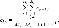 (4)
(4) - Define the feature-diversity score as:
.jpg "figure-protocol-5") . Interpret a larger db,v as lower mean similarity and greater diversity among the slice features, and a smaller db,v as greater feature redundancy. Therefore, for a batch containing B participants, obtain one diversity-score vector for each view: dv = [d1,v,d2,v,…,dB,v] ∈ RB.
. Interpret a larger db,v as lower mean similarity and greater diversity among the slice features, and a smaller db,v as greater feature redundancy. Therefore, for a batch containing B participants, obtain one diversity-score vector for each view: dv = [d1,v,d2,v,…,dB,v] ∈ RB. - Expand their shape from [B] to [B,1] and directly enter them into the adaptive sparsity controller.
- Configure the adaptive sparsity controller as a two-layer multilayer perceptron consisting of a linear layer from 1 to 128 dimensions, a ReLU activation, a linear layer from 128 to 1 dimension, and apply the Sigmoid function to obtain the scalar weight .
- Calculate the adaptive keep ratio as:
adaptive_keep_ratio=clamp(base_keep_ratio + (1-base_keep_ratio)qb,v,0.45,0.9) (5)
where denotes the baseline slice retention ratio.
The scaling factor is not independently tuned; it is defined as α = 1 − base_keep_ratio. With base_keep_ratio = 0.45, α = 0.55.
- Aggregate sparse and dense attention features
Aggregate slice features using parallel sparse and dense attention pathways. The sparse pathway selects the most informative slices for efficient aggregation, while the dense pathway preserves information from all slices. Fuse the two pathways through a residual connection to improve robustness.- For each sample in the batch, dynamically determine the number of retained slices K=int(Mv⋅adaptive_keep_ratio), according to its adaptive_keep_ratio.
- Compute sparse attention features, assign attention weights to the selected slices according to equation (6).
 (6)
(6)
where τ1 denotes the temperature parameter. - Obtain the sparse view-level feature by weighted summation of the selected slice features, as shown in equation (7):
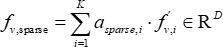 (7)
(7) - Compute dense attention features, assign attention weights to all Mv slices according to equation (8).
 (8)
(8) - Obtain the dense view-level feature by weighted summation of all slice features, as shown in equation (9):
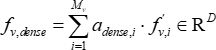 (9)
(9) - Fuse the sparse and dense aggregation features through a residual connection using a learnable parameter β ∈ [0,1] . Compute the final view-level aggregated feature according to Equation (10):
fv,aggregated =fv,sparse+ β⋅fv,dense ∈ RD (10) - Apply shared layer normalization and linear projection to map each aggregated view-level feature from 768 to 512 dimensions for subsequent multiview and whole-brain feature fusion.
- Extract whole-brain volumetric features using a 3D-CNN network
- Input each preprocessed whole-brain MRI volume into the CNN_Bone backbone to extract three-dimensional volumetric features. Use the network architecture summarized in Table 2.
- Construct CNN_Bone using four sequential ConvLayer modules. In each module, apply three-dimensional convolution, three-dimensional max pooling, batch normalization, and ReLU activation according to the parameters listed in Table 2. Progressively increase the feature-channel number from num to 8 × num, while reducing the spatial dimensions through max pooling.
- Retain the batch dimension and flatten all channel and spatial dimensions of the feature map output by the fourth ConvLayer into a one-dimensional feature vector.
- Apply Layer Normalization and linear projection to map the flattened feature vector to 512 dimensions for subsequent multiview and whole-brain feature fusion.
- Fuse multidimensional features using an adaptive gating module
Use an adaptive gating module to fuse multiview slice features and whole-brain volumetric features. The fusion process consists of three steps: feature quality assessment, adaptive gating weight generation, and weighted feature fusion. By dynamically assigning fusion weights to different feature dimensions, the module enables the model to emphasize more informative representations for each subject.- Assess feature quality
- Obtain four 512-dimensional feature vectors from the previous stage fx, fy, fz, f3D ∈ R512. Apply L2 normalization to all feature vectors before feature fusion, using 10-6 for numerical stability.
- Assign structurally identical but independently parameterized feature-informativeness assessors Qv to the four branches. Configure each assessor as a linear layer from 512 to 128 dimensions, a GELU activation, a linear layer from 128 to 1 dimension, and a sigmoid output.
sv = Qv (fv) ∈ (0,1) (11)
Define sv as the feature-informativeness score of the branch for diagnostic classification.
NOTE: The feature-informativeness score is learned through the classification cross-entropy loss without independent image-quality labels. - Concatenate the four branch scores into a four-dimensional score vector:
S = [sx,sy,sz,s3D] ∈ R4
- Generate adaptive gating weights
- Enter the score vector S into the gating network Gnet . Configure Gnet as a linear layer from 4 to 16 dimensions, a ReLU activation, and a linear layer from 16 to 4 dimensions. The gating network generate raw gating logits, as shown in equation (12):
Logits = Gnet(S) ∈ R4 (12) - Apply temperature-scaled Softmax across the four branches to obtain nonnegative gating weights that sum to 1.
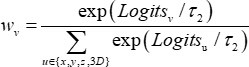 (13)
(13)
- Enter the score vector S into the gating network Gnet . Configure Gnet as a linear layer from 4 to 16 dimensions, a ReLU activation, and a linear layer from 16 to 4 dimensions. The gating network generate raw gating logits, as shown in equation (12):
- Perform adaptive feature fusion
- Calculate the weighted sum of the four normalized branch features.
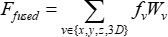 (14)
(14)
Use Ffused as the final fused feature representation.
- Calculate the weighted sum of the four normalized branch features.
- Assess feature quality
- Train and evaluate MDFAG-Net
- Train MDFAG-Net
- Partition the 842 subjects at the subject level using stratified sampling according to the NC, MCI, and AD labels and a random seed of 42. Assign subjects to the original training, validation, and independent test sets, respectively. Report the diagnostic-class distributions and proportions in Table 3.
- Keep the axial, coronal, and sagittal slices and the 3D MRI volume from each subject in the same data subset to prevent subject-level data leakage.
- Merge the original training and validation sets to form a development set of 674 subjects. Divide the development set into five folds at the subject level, using four folds for training and one fold for internal validation in each iteration.
- Implement MDFAG-Net using PyTorch on a workstation equipped with an NVIDIA GPU with 32 GB of memory. Set the random seed to 42.
- Train MDFAG-Net for 50 epochs using the Adam optimizer, an initial learning rate of 1 × 10⁻⁴ , a batch size of 16, and the cross-entropy loss function.
- Initialize τ1, γ , β, and base_keep_ratio in the Enhanced Sparse MIL module to 1.2, 0.5, 0.3, and 0.45, respectively. Restrict the adaptive keep ratio to 0.45–0.9, and τ2 initialize in the adaptive gating module to 1.0.
- Determine the principal hyperparameters using only the internal-validation data, and retain the setting achieving the highest validation accuracy. Keep the independent test set excluded from hyperparameter selection and model training.
- Save the model checkpoint achieving the highest internal-validation accuracy in each fold.
- Evaluate classification performance
- Load the checkpoint with the highest internal-validation accuracy from each fold and evaluate it on the fixed independent test set.
- Calculate accuracy, macro-averaged precision, macro-averaged recall, macro-averaged F1 score, and macro-averaged AUC(OvR). Calculate accuracy, precision, recall, and F1 score using Equations (15)–(18).
 (15)
(15)
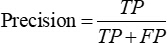 (16)
(16)
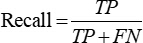 (17)
(17)
 (18)
(18) - Construct each comparison model according to its original publication, official public implementation, or standard-framework implementation, and retrain or fine-tune it using the training data in the present study. Retain the original network architecture and modify only the input interface and classification head required for the NC/MCI/AD three-class classification task. Report the implementation source, input configuration, initialization, task-specific adaptation, and selected learning rate of each method in Table 43,5,8–10,13,15,16,20–22.
- Evaluate all comparison methods using the same subject-level data partitions, MRI preprocessing pipeline, five-fold cross-validation procedure, independent test set, and evaluation metrics. Fix the optimizer category, batch size, loss function, maximum number of training epochs, and random seed across all methods.
- Apply the same prespecified candidate set {1×10-5,5×10-5,1×10-4,5×10-4} of initial learning rates to all methods. Select the final learning rate and model checkpoint exclusively according to the highest internal-validation accuracy in each fold. Do not use the independent test set for hyperparameter tuning or model selection.
- Define the macro-averaged AUC as the primary metric for statistical comparison. Compare each baseline method with MDFAG-Net using a two-sided paired t-test based on the fold-matched macro-AUC results. Report the exact p-values and define statistical significance as p < 0.05.
- Train MDFAG-Net
4.Perform hyperparameter sensitivity analysis
- Perform one-factor-at-a-time sensitivity analyses for base_keep_ratio, τ1, and τ2 on the development set using the same five-fold cross-validation protocol as the main experiments. Vary one parameter at a time while keeping the network architecture, data splits, and remaining training settings unchanged.
- Set base_keep_ratio sequentially to {0.30,0.35,0.40,0.45,0.50,0.55} . Evaluate τ1 and τ2 separately at {0.6,0.8,1.0,1.2,1.4,1.6}. Complete five-fold training and internal validation for each parameter setting, and record the Accuracy and Macro-AUC.
- For each τ1setting, extract the normalized attention weights of the retained slices generated by Equation (6) in the Enhanced Sparse MIL module. For a single view containing Kretained slices, calculate the normalized attention entropy as:
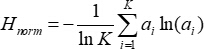 (19)
(19)
where ai denotes the normalized attention weight of the i-th retained slice, K denotes the actual number of retained slices. - Calculate the entropy-based attention sparsity index as: Satt=1-Hnorm , where a higher Satt indicates a more concentrated and sparse attention distribution, whereas a lower value indicates a more uniform attention distribution.
5.Perform model interpretability analysis
- Perform slice-level multiview Grad-CAM analysis
- Process all valid axial, coronal, and sagittal MRI slices in their original anatomical order using the corresponding ViT and Enhanced Sparse MIL modules. For each subject and view, determine the retained slices according to the slice-importance ranking and adaptive_keep_ratio.
- Summarize the adaptive keep ratio and the actual number of retained slices separately for the axial, coronal, and sagittal views, and further stratify the results by the NC, MCI, and AD diagnostic groups.
- Randomly select one subject from each diagnostic group using a fixed random seed. For each selected subject, select the retained slice with the highest slice-importance score from each anatomical view.
- Generate the Grad-CAM41 maps using the final Transformer encoder layer. Remove the CLS token, reshape the remaining 196 patch tokens into a 14 × 14 two-dimensional spatial layout, and resize the maps to 224 × 224 using nearest-neighbor interpolation. Normalize each map individually and overlay it on the corresponding MRI slice using semi-transparent visualization.
- Use the Hammersmith 95-region atlas to identify the anatomical regions corresponding to each selected slice. Calculate the mean normalized Grad-CAM response within each region and identify the region with the highest response. Compare the identified regions with previously reported Alzheimer’s disease-associated structures to assess the biological plausibility of the selected high-importance slices.
- Perform anatomy-based 3D whole-brain DeepSHAP analysis
- Load the trained MDFAG-Net model and process all subjects in the test set in evaluation mode. Using a fixed random seed, randomly select five MRI volumes from the NC subjects in the training set as a common reference background, and use the same background set for all DeepSHAP computations.
- For each subject, precompute and fix the axial, coronal, and sagittal features, and use only the 3D MRI volume as the input to be explained.
- Use block2conv of the 3D CNN branch as the intermediate explanation layer6,42. Calculate class-specific SHAP values for the NC, MCI, and AD outputs and convert them into three-dimensional attribution volumes.
- Map the attribution volumes to the preprocessed MRI space and parcellate the whole brain using the Hammersmith 95-region atlas. Sum the absolute voxel-level SHAP values within each region to obtain region-level attribution scores.
- Group the test subjects according to their predicted classes. Average the corresponding class-specific regional scores within the predicted MCI and AD cohorts, rank the 95 regions in descending order, and display the 15 highest-contributing regions for each cohort.
תוצאות
Classification performance comparison
Perform anatomy-based 3D whole-brain DeepSHAP analysis
The classification performance of MDFAG-Net was compared with representative MRI-based methods for Alzheimer’s disease classification, including 3D-CNN, ResNet34, DenseNet121, PlgFormer, PDMML, 3D Swin Transformer, 2D-CNN, ViT, BrainMAE, MSA3D, and PMF-Net. All methods were evaluated on the same ADNI cohort using identical subject-level data partitions and evaluation metrics, following the implementation and hyperparameter-tuning procedures described in the Protocol. The quantitative results are presented in Table 53,5,8,9,10,13,15,16,20,21,22.
As shown in Table 5, MDFAG-Net achieved the best overall classification performance, with an accuracy of 0.661 ± 0.027, a precision of 0.683 ± 0.030, an F1-score of 0.658 ± 0.020, and a macro-AUC of 0.798 ± 0.030, together with a recall of 0.650 ± 0.030. These results demonstrate the benefit of jointly exploiting multiview 2D slice representations and whole-brain 3D structural features for AD classification.
Compared with the traditional 3D-CNN, MDFAG-Net improved the accuracy from 0.609 to 0.661 and the F1-score from 0.592 to 0.658. Relative to ViT, MDFAG-Net increased the accuracy, F1-score, and macro-AUC from 0.641, 0.643, and 0.782 to 0.661, 0.658, and 0.798, respectively. Compared with 3D Swin Transformer, BrainMAE, and PMF-Net, MDFAG-Net improved the macro-AUC by 0.017, 0.009, and 0.014, respectively, further supporting the effectiveness of jointly modeling multiview slice information and whole-brain 3D structural information. Two-sided paired t-tests based on the fold-matched macro-AUC results showed statistically significant improvements over 3D-CNN, ResNet34, PDMML, and 2D-CNN. Although MDFAG-Net also achieved higher mean macro-AUC values than the remaining methods, these differences did not reach statistical significance (Table 5).
Regarding class-specific discriminative ability, the ROC curves shown in Figure 6 yielded AUC(OvR) values of 0.825, 0.708, and 0.897 for NC, MCI, and AD, respectively, for MDFAG-Net. Notably, although MCI is typically characterized by relatively subtle structural alterations, MDFAG-Net achieved the highest MCI-specific AUC among the evaluated methods (0.708), exceeding ViT (0.696), BrainMAE (0.697), and 3D Swin Transformer (0.685). This finding suggests that jointly exploiting multiview 2D slice information and whole-brain 3D structural features may facilitate the identification of subtle structural differences associated with MCI.
Ablation studies
Hyperparameter sensitivity analysis
Hyperparameter sensitivity analyses were conducted to evaluate the effects of base_keep_ratio, , and on the performance of MDFAG-Net. Figure 7 shows the classification performance under different base_keep_ratio and settings, while Table 6 further reports the effect of on both classification performance and the distribution of slice-level attention weights.
As shown in Figure 7, variations in base_keep_ratio and affected model performance, although the overall fluctuations were relatively small. For base_keep_ratio, the best performance was obtained at 0.45; a lower retention ratio may discard informative slices, whereas further increasing the ratio provided no additional benefit, suggesting increased redundancy. For, the model performed best at 1.0, while deviations from this value generally reduced performance, indicating that a moderate temperature facilitates effective adaptive gating across feature dimensions. Overall, base_keep_ratio = 0.45 and .
Table 6 further shows the effect of on slice-level attention sparsity. As increased, progressively decreased, indicating that the attention weights became less concentrated across the retained slices. However, stronger sparsity did not necessarily result in better classification performance. The best performance was achieved at , whereas either lower or higher values resulted in reduced performance. These results indicate that an intermediate attention concentration provides a better balance between emphasizing informative slices and preserving complementary information. Therefore, was used in the final model.
Impact of different dimensions
In this experiment, the impact of different dimensions on the classification performance of the proposed MDFAG-Net framework was studied. While keeping the model architecture and training strategy unchanged, different 2D slice dimensions on the basis of the original 3D MRI dimensions were added. The changes in model performance to quantify the contribution of each dimension were evaluated, as shown in Figure 8.
As shown in Figure 8, the MDFAG-Net model achieved the best performance across all evaluation indicators, fully verifying the effectiveness of the proposed multidimensional fusion strategy. In contrast, the performance of the 3D-CNN baseline model, which relies only on 3D MRI data, is relatively low, indicating that pure 3D imaging has limitations in capturing subtle pathological features. When the single-view 2D slice sequence was introduced into the 3D-CNN baseline model, its performance was improved to varying degrees. This clearly shows that 2D slice images from different perspectives can provide unique and complementary diagnostic information for 3D MRI data. Overall, the MDFAG-Net model that fully integrates all modalities is better than any combination model that relies only on a single 2D perspective. This emphasizes that integrating multidimensional information can achieve a more comprehensive and robust feature representation, which is crucial to improving the classification performance.
Impact of the enhanced sparse MIL aggregation module
We used Enhanced Sparse MIL in the MDFAG-Net model to fully model the correlation between slices at the slice-level feature extraction stage, so as to effectively distinguish between key focal slices and unrelated or noise slices. In this subsection, an ablation experiment was designed to verify the effectiveness of the aggregation module by removing the module from MDFAG-Net and naming the modified model MDFAG-Net-1, as shown in Figure 9.
As shown in Figure 9, MDFAG-Net outperformed MDFAG-Net-1 in all indicators. For example, the accuracy of MDFAG-Net reached 0.661, while MDFAG-Net-1 is 0.631. For AUC, MDFAG-Net reached 0.798, 3 percentage points higher than the 0.768 of MDFAG-Net-1. These results show that the Enhanced Sparse MIL aggregation module is crucial to the excellent performance of MDFAG-Net. Its multiscale scoring and adaptive sparse selection can more effectively filter and aggregate slice features with diagnostic value.
Impact of the adaptive gating module
We adopted adaptive gating technology in the MDFAG-Net model to adaptively adjust the contribution weight of each dimension in the multidimensional feature fusion stage. In order to verify the effectiveness of the adaptive gating module, an ablation experiment was designed to remove the module from MDFAG-Net and name the model obtained as MDFAG-Net-2, as shown in Figure 10.
As shown in Figure 10, the performance comparison of MDFAG-Net and MDFAG-Net-2 in NC/MCI/AD multiclassification tasks shows that the adaptive gating module has a positive impact on the performance of the model. Although the improvement of these individual indicators is not as significant as that of the aggregation mechanism, the adaptive gating module has enhanced all key indicators. These results show that the adaptive gating module optimizes the integration process of multidimensional information. By dynamically adjusting the contribution of each dimension, the model significantly improves its ability to classify Alzheimer's disease.
Model interpretability analysis
Slice-level multiview Grad-CAM analysis
To characterize the adaptive slice-selection behavior of the Enhanced Sparse MIL module, the adaptive keep ratio and the actual number of retained slices were summarized separately for the axial, coronal, and sagittal views across the NC, MCI, and AD groups (Table 7).
As shown in Table 7, the slice retention ratios varied across diagnostic groups and anatomical views, reflecting the adaptive selection of informative slices by the Enhanced Sparse MIL module.
To further assess the anatomical relevance of the selected high-importance slices, Grad-CAM analysis was performed on representative high-importance slices from the three diagnostic groups (Figure 11). Distinct spatial response patterns were observed across diagnostic groups and anatomical views. Responses in the NC group were relatively dispersed and mainly involved cortical and some periventricular regions. The MCI group showed more concentrated responses in the periventricular and medial cortical regions, whereas the AD group exhibited more extensive responses involving the periventricular and medial cortical regions.
Further region-based analysis using the Hammersmith 95-region atlas localized the high Grad-CAM responses primarily to the posterior cingulate gyrus, precuneus, and medial frontal regions. These regional findings were spatially consistent with the medial cortical responses observed in the high-importance slices. In particular, the posterior cingulate and precuneus are among the medial cortical structures frequently implicated in AD-related structural alterations43,44,45. Together, the anatomical distribution of the Grad-CAM responses and the atlas-based regional localization indicate that the high-importance slices selected by the Enhanced Sparse MIL module contain information about AD-associated brain structural alterations, thereby supporting the biological plausibility of the adaptive slice-selection mechanism.
Anatomy-based 3D whole-brain SHAP analysis
DeepSHAP attribution analysis was performed with normal-control samples as the baseline, following the computational workflow described in the Protocol. The Hammersmith 95-region atlas was used to aggregate voxel-wise SHAP values into regional attribution scores, and the top 15 contributing brain regions were identified for MCI-predicted and AD-predicted test subjects (Figure 12).
As shown in Figure 12, in the MCI group (Figure 12A), the attribution weights of the 3D CNN branch are primarily dominated by the Left/Right lateral ventricle posterior part and the Left/Right posterior cingulate gyrus. As a core brain region of the default mode network (DMN), the high attribution proportion of the posterior cingulate gyrus indicates that the system's decision-making relies heavily on the specific network topological degradation features during the prodromal phase46. In addition, the Left/Right amygdala, Left/Right hippocampus, Left/Right parahippocampal gyrus anterior part, and Left/Right anterior cingulate gyrus also ranked among the top, directly providing a quantitative characterization of medial temporal lobe atrophy and limbic system damage during the MCI stage.
In contrast, in the AD group (Figure 12B), the spatial distribution of SHAP scores exhibits a combined characteristic of brain parenchyma atrophy and ventricular enlargement. Compared with the MCI group, the attribution weights of the Left/Right amygdala and Left hippocampus/Right hippocampus increase significantly, corresponding to the typical anatomical features of medial temporal lobe atrophy in clinical AD47. Simultaneously, the system's attention is widely distributed across the ventricular system; except for the Left/Right lateral ventricle posterior part, the rankings of the Left/Right lateral ventricle anterior part and the Left/Right temporal horn of the lateral ventricle both increase. The aforementioned statistical results at the group level highly conform to the classic pathological imaging characteristics of “medial temporal lobe atrophy combined with compensatory holoventricular enlargement” in AD patients45.
The complete MDFAG-Net implementation, including data preparation, Enhanced Sparse MIL, adaptive gating, model training and evaluation, Grad-CAM visualization, and DeepSHAP analysis, is available at GitHub: https://github.com/MDFAG-Net/MDFAG-Net.
Data analyzed in this study were obtained from the Alzheimer’s Disease Neuroimaging Initiative (ADNI) database. ADNI data are hosted by the LONI Image and Data Archive (IDA). Researchers must complete academic registration and accept the ADNI data‑use agreement to gain access. The main project portal is available at https://adni.loni.usc.edu/, and the data‑access application page is at https://ida.loni.usc.edu/collaboration/access/appLicense.jsp. No universal dataset‑level DOI or accession identifier exists for the full ADNI repository. The processed derivative data generated in this study are not essential for reproducing the study’s analyses and results, as they can be regenerated from the original ADNI data using the procedures described in this protocol.
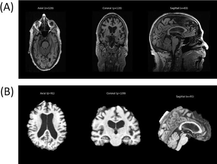
Figure 1: Comparison of original and preprocessed brain MRI slices (Axial/Coronal/Sagittal). (A) Before preprocessing. (B) After preprocessing. Please click here to view a larger version of this figure.
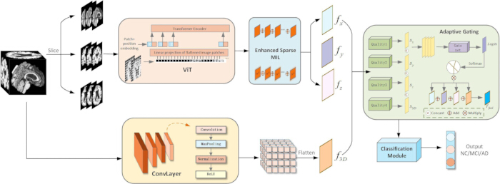
Figure 2: Overall architecture of MDFAG-Net. The framework integrates multiview slice-level representations and whole-brain structural features for NC/MCI/AD classification through enhanced sparse MIL aggregation and adaptive gating-based feature fusion. Please click here to view a larger version of this figure.
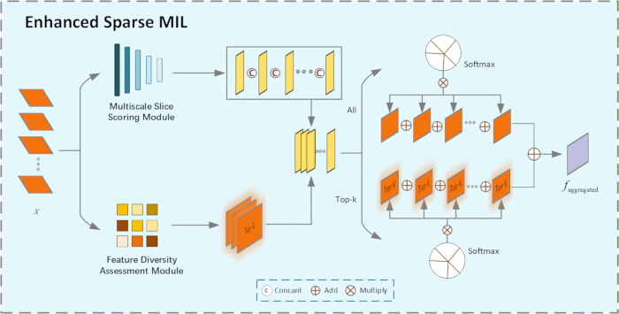
Figure 3: Structure of the enhanced sparse MIL aggregation module. Slice importance and feature diversity are jointly evaluated to perform adaptive Top-k selection. The selected slices and all candidate slices are aggregated through sparse and dense pathways to obtain the final representation. Please click here to view a larger version of this figure.
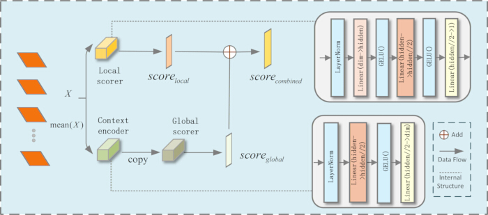
Figure 4: Structure of the multiscale slice scoring module. Local slice information and global contextual information are jointly modeled to generate the final slice-importance score used for slice ranking. Please click here to view a larger version of this figure.
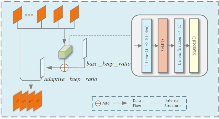
Figure 5: Structure of the feature diversity assessment module. Feature diversity among slices is estimated and combined with the base_keep_ratio to determine the adaptive_keep_ratio for Top-k selection. Please click here to view a larger version of this figure.
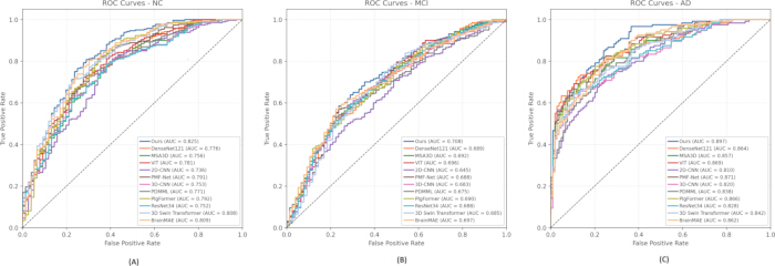
Figure 6: ROC curves for different competitive methods across categories. (A) NC (B) MCI (C) AD. The curves show one-vs-rest receiver operating characteristic (ROC) performance, with the corresponding area under the curve (AUC) reported for each method. Please click here to view a larger version of this figure.
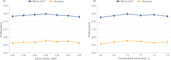
Figure 7: Hyperparameter sensitivity analysis of MDFAG-Net. Macro-AUC and accuracy are compared under different (A) base_keep_ratio and (B) temperature parameter settings. Error bars indicate the variability across the five folds. Please click here to view a larger version of this figure.
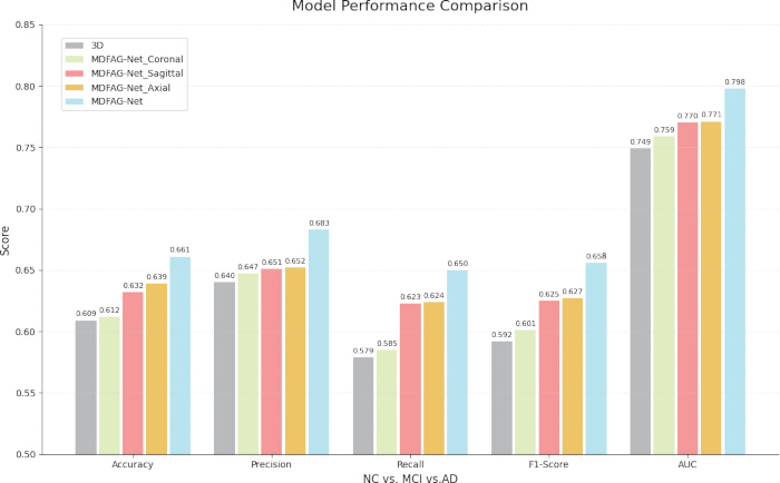
Figure 8: Impact of different feature dimensions on classification performance. The 3D-only, single-view axial, coronal, and sagittal configurations are compared with the complete MDFAG-Net using Accuracy, Precision, Recall, F1-score, and AUC. Please click here to view a larger version of this figure.
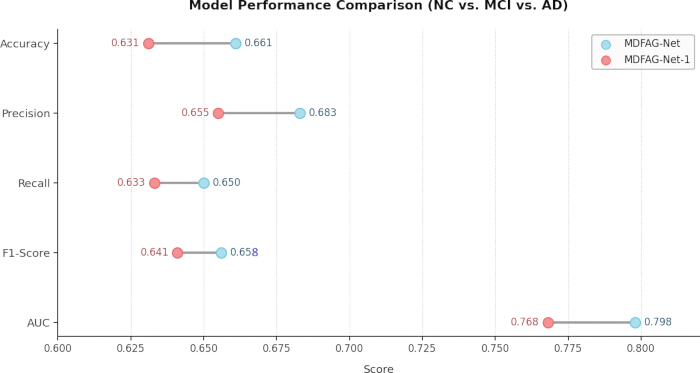
Figure 9: Impact of the enhanced sparse MIL aggregation module. Classification performance of the complete MDFAG-Net is compared with that of the model without the enhanced sparse MIL module across five evaluation metrics. Please click here to view a larger version of this figure.
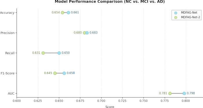
Figure 10: Impact of the adaptive gating module. Classification performance of the complete MDFAG-Net is compared with that of the model without adaptive gating across five evaluation metrics.Please click here to view a larger version of this figure.
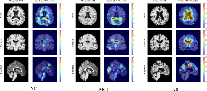
Figure 11: Grad-CAM visualization saliency maps across multiple orthogonal planes for NC, MCI, and AD subjects. From left to right, representative cases of NC, MCI, and AD are presented. Each row corresponds to the Axial, Coronal, and Sagittal planes, respectively. In each pair, the left image shows the original MRI, while the right image displays the Grad-CAM overlay. Please click here to view a larger version of this figure.
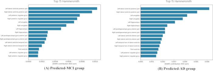
Figure 12: Population-level anatomical brain region contributions based on DeepSHAP. (A) Top 15 ROIs ranked by absolute SHAP scores in the predicted-MCI group. (B) Top 15 ROIs ranked by absolute SHAP scores in the predicted-AD group. The x-axis denotes the accumulated absolute SHAP value per region based on the Hammersmith atlas, representing the macroscopic attribution of the 3D CNN branch. Please click here to view a larger version of this figure.
| Category | Gender(Male/Female) | Age (years) | Weight (kg) |
| AD | 141/99 | 75.81 ± 7.92 | 74.34 ± 15.33 |
| MCI | 167/89 | 75.97 ± 7.47 | 76.47 ± 14.85 |
| NC | 174/172 | 75.43 ± 5.87 | 76.05 ± 15.26 |
Table 1: Clinical information of ADNI study participants. Demographic and clinical characteristics of participants in the NC, MCI, and AD groups are summarized.
| Block | Input Channels | Output Channels | Convolution (Kernel/Stride) | Pooling(Kernel/Stride) | Normalization & Activation |
| 1 | 1 | num | Conv(7/2) | Pool(3/2) | BN + ReLU |
| 2 | num | 2 * num | Conv(4/1) | Pool(2/2) | BN + ReLU |
| 3 | 2 * num | 4 * num | Conv(3/1) | Pool(2/2) | BN + ReLU |
| 4 | 4 * num | 8 * num | Conv(3/1) | Pool(2/2) | BN + ReLU |
Table 2: Structural parameters of the CNN_Bone backbone network. The architecture and parameter settings of the four ConvLayer blocks used for whole‑brain 3D feature extraction are summarized. Here, “num” denotes the configurable base number of output channels; num was set to 20 in the experiments reported in this study.
| Data subset | NC | MCI | AD | Total | Proportion |
| Original training set | 242 | 179 | 168 | 589 | 70.00% |
| Original validation set | 35 | 26 | 24 | 85 | 10.00% |
| Independent test set | 69 | 51 | 48 | 168 | 20.00% |
| Total | 346 | 256 | 240 | 842 | 100.00% |
Table 3: Dataset partition for NC, MCI, and AD subjects. The numbers and proportions of NC, MCI, and AD subjects in the training, validation, and independent test sets are reported.
| Method | Implementation source | Input configuration | Selected learning rate |
| 3D-CNN [8] | Reproduced using the authors’ publicly available code | 3D T1-weighted MRI | 5 × 10⁻⁴ |
| ResNet34 [9] | Reproduced using the authors’ publicly available code | 3D T1-weighted MRI | 1 × 10⁻⁴ |
| DenseNet121 [10] | Reproduced using the authors’ publicly available code | 3D T1-weighted MRI | 1 × 10⁻⁴ |
| PlgFormer [13] | Reimplemented in-house based on the original publication | 3D T1-weighted MRI | 5 × 10⁻⁴ |
| 3D Swin Transformer [15] | Reproduced using the authors’ publicly available code | 3D T1-weighted MRI | 5 × 10⁻⁴ |
| BrainMAE [16] | Reproduced using the authors’ publicly available code and pretrained weights | 3D T1-weighted MRI | 1 × 10⁻⁴ |
| PDMML [3] | Reproduced using the authors’ publicly available code | Local 3D MRI patches | 1 × 10⁻⁴ |
| 2D-CNN [20] | Reproduced using the authors’ publicly available code | Axial, coronal, and sagittal MRI slices | 5 × 10⁻⁴ |
| ViT [21] | Reproduced using the authors’ publicly available code | Multi-view MRI slices resized to 224 × 224 | 5 × 10⁻⁴ |
| PMF-Net [22] | Reimplemented in-house based on the original publication | Axial, coronal, and sagittal MRI slices | 1 × 10⁻⁴ |
| MSA3D [5] | Reimplemented in-house based on the original publication | Multi-view 2D MRI slices and 3D T1-weighted MRI | 1 × 10⁻⁴ |
Table 4: Implementation details of the comparison methods. The implementation source, input configuration, and selected learning rate are provided for each comparison method.
| Method | Accuracy | Precision | Recall | F1-Score | AUC | P‑value |
| 3D-CNN [8] | 0.609 ± 1.3% | 0.640 ± 0.01 | 0.579 ± 0.01 | 0.592 ± 0.01 | 0.749 ± 0.02 | 0.021 |
| ResNet34 [9] | 0.620 ± 1.2% | 0.641 ± 0.03 | 0.620 ± 0.01 | 0.619 ± 0.01 | 0.754 ± 0.01 | 0.028 |
| DenseNet121 [10] | 0.631 ± 2.2% | 0.649 ± 0.04 | 0.632 ± 0.03 | 0.642 ± 0.03 | 0.771 ± 0.03 | 0.104 |
| PlgFormer [13] | 0.639 ± 2.2% | 0.664 ± 0.04 | 0.637 ± 0.03 | 0.649 ± 0.03 | 0.782 ± 0.03 | 0.237 |
| 3D Swin Transformer [15] | 0.641 ± 2.0% | 0.661 ± 0.03 | 0.636 ± 0.03 | 0.647 ± 0.02 | 0.781 ± 0.02 | 0.146 |
| PDMML [3] | 0.640 ± 1.9% | 0.659 ± 0.03 | 0.649 ± 0.02 | 0.654 ± 0.03 | 0.762 ± 0.01 | 0.043 |
| 2D-CNN [20] | 0.614 ± 2.1% | 0.636 ± 0.03 | 0.619 ± 0.02 | 0.620 ± 0.02 | 0.731 ± 0.02 | 0.011 |
| BrainMAE [16] | 0.653 ± 1.6% | 0.672 ± 0.02 | 0.651 ± 0.02 | 0.657 ± 0.02 | 0.789 ± 0.02 | 0.381 |
| ViT [21] | 0.641 ± 1.6% | 0.663 ± 0.02 | 0.647 ± 0.02 | 0.643 ± 0.02 | 0.782 ± 0.01 | 0.129 |
| PMF-Net [22] | 0.646 ± 2.2% | 0.671 ± 0.02 | 0.643 ± 0.01 | 0.652 ± 0.02 | 0.784 ± 0.02 | 0.264 |
| MSA3D [5] | 0.637 ± 2.5% | 0.651 ± 0.02 | 0.646 ± 0.03 | 0.641 ± 0.01 | 0.769 ± 0.02 | 0.053 |
| This study | 0.661 ± 2.7% | 0.683 ± 0.03 | 0.650 ± 0.03 | 0.658 ± 0.02 | 0.798 ± 0.03 | — |
Table 5: Classification performance of different methods on the ADNI dataset. Results are reported as mean ± standard deviation across five folds. The p-values represent paired comparisons of fold‑matched macro‑AUC values between each method and MDFAG‑Net.
| τ1 | Satt | Accuracy | AUC |
| 0.6 | 0.438 ± 0.05 | 0.644 ± 0.03 | 0.781 ± 0.02 |
| 0.8 | 0.379 ± 0.04 | 0.653 ± 0.02 | 0.789 ± 0.03 |
| 1.0 | 0.334 ± 0.05 | 0.651 ± 0.02 | 0.787 ± 0.02 |
| 1.2 | 0.292 ± 0.04 | 0.661 ± 0.03 | 0.798 ± 0.03 |
| 1.4 | 0.257 ± 0.03 | 0.656 ± 0.02 | 0.792 ± 0.04 |
| 1.6 | 0.229 ± 0.04 | 0.649 ± 0.04 | 0.785 ± 0.02 |
Table 6: Effect of the temperature parameter on model performance and attention sparsity. Classification performance and slice‑level attention sparsity under different temperature settings are reported.
| Diagnostic group | View | Adaptive _keep_ratio | Retained slices |
| NC | Sagittal | 0.68 ± 0.06 | 33.3 ± 2.8 |
| NC | Coronal | 0.71 ± 0.06 | 34.8 ± 3.0 |
| NC | Axial | 0.65 ± 0.04 | 31.9 ± 2.0 |
| MCI | Sagittal | 0.74 ± 0.07 | 36.3 ± 3.2 |
| MCI | Coronal | 0.66 ± 0.05 | 32.4 ± 2.5 |
| MCI | Axial | 0.71 ± 0.05 | 34.8 ± 2.3 |
| AD | Sagittal | 0.69 ± 0.07 | 33.8 ± 3.5 |
| AD | Coronal | 0.72± 0.08 | 35.3 ± 3.7 |
| AD | Axial | 0.73± 0.04 | 35.8 ± 1.9 |
Table 7: Adaptive slice retention across diagnostic groups and anatomical views. Adaptive keep ratios and the corresponding numbers of retained slices are reported for the sagittal, coronal, and axial views across the NC, MCI, and AD groups.
דיון
The proposed MDFAG-Net achieved improved classification performance compared with representative 2D, 3D, and multibranch methods on the ADNI dataset. Ablation experiments demonstrated the contributions of Enhanced Sparse MIL and Adaptive Gating, supporting the effectiveness of adaptive slice aggregation and dynamic 2D–3D feature fusion. Grad-CAM and DeepSHAP further highlighted anatomically meaningful structures, including the hippocampus, amygdala, posterior cingulate gyrus, parahippocampal gyrus, and ventricular system43,44,45,46,47.
Compared with conventional 2D methods that provide limited volumetric context20,21,22,23,24 and whole-volume 3D methods that directly model volumetric structure8,9,10,11,12,13,14,15,16, MDFAG-Net jointly models multiview slice-level and whole-brain 3D representations. Enhanced Sparse MIL adaptively emphasizes informative slices while preserving global slice information, whereas Adaptive Gating dynamically balances heterogeneous feature branches rather than relying on fixed fusion weights. The framework is therefore particularly useful when complementary multiview information, whole-brain structural context, and interpretable prediction are jointly required, although its multibranch design increases model complexity.
Preprocessing and slice selection are critical to reliable implementation. Image orientation, brain extraction, spatial registration, mid-slice position, and anatomical coverage of candidate slices should be visually verified before training. If the adaptive keep ratio frequently approaches its predefined bounds, the feature-diversity distribution and sparsity-controller output should be examined, and the base keep ratio may be recalibrated on the validation set. Excessively concentrated or diffuse attention may indicate that the temperature parameter requires adjustment. If one anatomical view consistently dominates the fusion weights, registration accuracy, valid slice coverage, and branch-specific feature distributions should first be examined. When computational resources are limited, the number of candidate slices or model complexity may be reduced, but these modifications should be re-evaluated on the validation set.
The principal limitations are the single-dataset evaluation, the computational cost of the multibranch architecture, and potential dependence on preprocessing and anatomical parcellation. The FSL-based brain extraction and spatial registration may affect anatomical correspondence, candidate slice distribution, slice-importance estimation, and whole-brain feature extraction. Similarly, regional attribution based on the Hammersmith 95-region atlas depends on image-to-atlas registration and parcellation definitions and may vary with alternative atlases. Although alternative preprocessing pipelines and anatomical atlases can be incorporated without changing the overall MDFAG-Net architecture, robustness to these choices has not yet been systematically established. In addition, Grad-CAM and DeepSHAP indicate regions associated with model predictions rather than direct evidence of disease-specific pathological changes.
Future work should evaluate MDFAG-Net on independent multicenter datasets and systematically examine its robustness across preprocessing pipelines and anatomical atlases. Further studies may also investigate more efficient implementations and assess the reproducibility of adaptive slice selection and regional attribution. Extension to longitudinal or multimodal neuroimaging data may further determine the applicability of the framework beyond single-time-point structural MRI.
In summary, MDFAG-Net provides a flexible framework for integrating multiview slice-level and whole-brain structural representations for sMRI-based AD classification. Its combination of adaptive slice aggregation, dense information preservation, and dynamic multidimensional feature fusion enables complementary modeling of localized and distributed structural information. The framework may be particularly useful when multiview information, adaptive slice selection, and interpretable subject-level prediction are jointly required. Further validation across independent datasets, preprocessing strategies, and anatomical parcellation schemes is needed to establish its generalizability and robustness.
גילויים
The authors declare that they have no conflicts of interest. No generative AI tools were employed in the preparation of the manuscript, development of the code, analysis of the data, or preparation of the figures.
AUTHOR CONTRIBUTIONS:
Conceptualization, Y.Z. and Q.Z.; methodology, L.Z., Y.Z. and Q.Z.; software, L.Z. and Y.Z.; validation, L.Z.; formal analysis, L.Z.; investigation, Q.Z., J.W.; resources, Y.Z.; data curation, L.Z.; writing—original draft preparation, L.Z.; writing—review and editing, Y.Z.; visualization, L.Z.; supervision, Y.Z.; project administration, Y.Z. and Z.L.; funding acquisition, Y.Z. and Q.Z. All authors have read and agreed to the published version of the manuscript
תודות
This research was funded by the National Natural Science Foundation of China under (Grant No. 62433002) and (Grant No. 62476014), the National Science and Technology Major Project (No. 2021ZD0113703), the Beijing Municipal Social Science Foundation Annual Planning Project (No. 23GLB014), the Project of Construction and Support for High-level Innovative Teams of Beijing Municipal Institutions under (Grant No. BPHR20220104), and the Beijing Scholars Program under (Grant No. 099).
חומרים
| שם | חברה | מספר קטלוג | הערות |
|---|---|---|---|
| Alzheimer's Disease Neuroimaging Initiative (ADNI) dataset | Alzheimer's Disease Neuroimaging Initiative | https://adni.loni.usc.edu/ | Source of T1-weighted structural MRI data for NC, MCI, and AD classification |
| FMRIB Software Library (FSL) | University of Oxford | Version 6.0 / https://fsl.fmrib.ox.ac.uk/fsl/docs/ | MRI preprocessing, including skull stripping, spatial registration, bias field correction, and brain segmentation |
| Hammersmith adult brain atlas (95 ROIs) | Imperial College London | https://brain-development.org/brain-atlases/adult-brain-atlases/ | Anatomical parcellation for ROI-based Grad-CAM and DeepSHAP analyses |
| Python | Python Software Foundation | Version 3.9 | Programming environment |
| PyTorch | PyTorch Foundation | PyTorch 2.1.0 | Deep learning framework used to implement and train MDFAG-Net |
| ViT-Base-Patch16-224-in21k | Google Research | https://github.com/google-research/vision_transformer | Pretrained Vision Transformer used for slice-level feature extraction |
| NVIDIA vGPU | NVIDIA | NVIDIA Tesla V100-SXM2-32G | GPU platform used for model training and inference |
מקורות
- Kim CM, et al. Amyloid beta-weighted cortical thickness: a new imaging biomarker in Alzheimer's disease. Curr Alzheimer Res. 2015;12(6):563–571.
- Ullah Z, Jamjoom M. A deep learning for Alzheimer's stages detection using brain images. Comput Mater Contin. 2023;74(1):1457–1473.
- Liu F, Yuan S, Li W, Xu Q, Sheng B. Patch-based deep multimodal learning framework for Alzheimer's disease diagnosis using multiview neuroimaging. Biomed Signal Process Control. 2023;80:104400.
- Veitch DP, et al. Using the Alzheimer's Disease Neuroimaging Initiative to improve early detection, diagnosis, and treatment of Alzheimer's disease. Alzheimers Dement. 2022;18(4):824–857.
- Chen L, Qiao H, Zhu F. Alzheimer's disease diagnosis with brain structural MRI using multiview-slice attention and 3D convolution neural network. Front Aging Neurosci. 2022;14:871706.
- Aliyu BS, et al. Enhanced feature selection for imbalanced microarray cancer gene classification using chaotic Salp swarm algorithm. Int J Theor Appl Comput Intell. 2025:258–283.
- Karimi M, et al. Feature selection methods in big medical databases: a comprehensive survey. Int J Theor Appl Comput Intell. 2025:181–209.
- Qiu S, et al. Multimodal deep learning for Alzheimer's disease dementia assessment. Nat Commun. 2022;13(1):3404.
- Korolev S, Safiullin A, Belyaev M, Dodonova Y. Residual and plain convolutional neural networks for 3D brain MRI classification. In: 2017 IEEE 14th International Symposium on Biomedical Imaging (ISBI); 2017. p. 835–838. doi:10.1109/ISBI.2017.7950647.
- Cui R, Liu M. Hippocampus analysis by combination of 3-D DenseNet and shapes for Alzheimer's disease diagnosis. IEEE J Biomed Health Inform. 2019;23(5):2099–2107.
- Ramzan F, Khan MUG, Iqbal S, Saba T, Rehman A. Volumetric segmentation of brain regions from MRI scans using 3D convolutional neural networks. IEEE Access. 2020;8:103697–103709.
- Tong Y, et al. Research of spatial context convolutional neural networks for early diagnosis of Alzheimer's disease. J Supercomput. 2024;80(4):5279–5297.
- Wang G, et al. PlgFormer: parallel extraction of local-global features for AD diagnosis on sMRI using a unified CNN-transformer architecture. Front Neurol. 2025;16:1626922.
- Ren F, Yang C, Nanehkaran YA. MRI-based model for MCI conversion using deep zero-shot transfer learning. J Supercomput. 2023;79(2):1182–1200.
- Tang Y, et al. Self-supervised pre-training of Swin Transformers for 3D medical image analysis. In: Proceedings of the IEEE/CVF Conference on Computer Vision and Pattern Recognition; 2022. p. 20730–20740. doi:10.1109/CVPR52688.2022.02007.
- Yang Y, Mao Y, Liu X, Liu X. BrainMAE: region-aware self-supervised learning framework for brain signals [Preprint]. arXiv. 2024. doi:10.48550/arXiv.2406.17086. Available from: https://arxiv.org/abs/2406.17086
- Ortiz A, Munilla J, Górriz JM, Ramírez J. Ensembles of deep learning architectures for the early diagnosis of Alzheimer's disease. Int J Neural Syst. 2016;26(7):1650025.
- Liu M, Zhang J, Adeli E, Shen D. Landmark-based deep multiinstance learning for brain disease diagnosis. Med Image Anal. 2018;43:157–168.
- Chen Y, Xia Y. Iterative sparse and deep learning for accurate diagnosis of Alzheimer's disease. Pattern Recognit. 2021;116:107944.
- Angkoso CV, Tjahyaningtijas HPA, Purnomo MH, Purnama IKE. Multiplane convolutional neural network (Mp-CNN) for Alzheimer's disease classification. Int J Intell Eng Syst. 2022;15(1):329–340.
- Alshayeji MH. Alzheimer's disease detection and stage identification from magnetic resonance brain images using vision transformer. Mach Learn Sci Technol. 2024;5(3):035011.
- Zhang Q, et al. A multislice attention fusion and multiview personalized fusion lightweight network for Alzheimer's disease diagnosis. BMC Med Imaging. 2024;24(1):258.
- Ban Y, Zhang X, Lao H. Diagnosis of Alzheimer's disease using structure highlighting key slice stacking and transfer learning. Med Phys. 2022;49(9):5855–5869.
- Pereira MEC, Fantini I, Lotufo RA, Rittner L. An extended-2D CNN for multiclass Alzheimer's disease diagnosis through structural MRI. Proc SPIE. 2020;11314:113141V. doi:10.1117/12.2550753.
- Qiao H, Chen L, Zhu F. A fusion of multiview 2D and 3D convolution neural network based MRI for Alzheimer's disease diagnosis. In: 2021 43rd Annual International Conference of the IEEE Engineering in Medicine & Biology Society (EMBC); 2021. p. 3317–3321. doi:10.1109/EMBC46164.2021.9629923. Available from: https://ieeexplore.ieee.org/document/9629923
- Chen Y, Pan Y, Xia Y, Yuan Y. Disentangle first, then distill: a unified framework for missing modality imputation and Alzheimer's disease diagnosis. IEEE Trans Med Imaging. 2023;42(12):3566–3578.
- Pan Y, Liu M, Xia Y, Shen D. Disease-image-specific learning for diagnosis-oriented neuroimage synthesis with incomplete multimodality data. IEEE Trans Pattern Anal Mach Intell. 2022;44(10):6839–6853.
- Ilse M, Tomczak JM, Welling M. Attention-based deep multiple instance learning. In: Proceedings of the 35th International Conference on Machine Learning; 2018. PMLR. 2018;80:2127–2136. Available from: https://proceedings.mlr.press/v80/ilse18a.html
- Courtiol P, Tramel EW, Sanselme M, Wainrib G. Classification and disease localization in histopathology using only global labels: a weakly-supervised approach [Preprint]. arXiv. 2018. doi:10.48550/arXiv.1802.02212. Available from: https://arxiv.org/abs/1802.02212
- Campanella G, et al. Clinical-grade computational pathology using weakly supervised deep learning on whole slide images. Nat Med. 2019;25(8):1301–1309.
- Martins AFT, Astudillo RF. From softmax to sparsemax: a sparse model of attention and multilabel classification. In: Proceedings of the 33rd International Conference on Machine Learning; 2016. PMLR. 2016;48:1614–1623. Available from: https://proceedings.mlr.press/v48/martins16.html
- Teerapittayanon S, McDanel B, Kung HT. BranchyNet: fast inference via early exiting from deep neural networks. In: 2016 23rd International Conference on Pattern Recognition (ICPR); 2016. p. 2464–2469. doi:10.1109/ICPR.2016.7900006.
- Shen J, et al. Fractional skipping: towards finer-grained dynamic CNN inference. Proc AAAI Conf Artif Intell. 2020;34(4):5700–5708.
- Xue Z, Marculescu R. Dynamic multimodal fusion. In: 2023 IEEE/CVF Conference on Computer Vision and Pattern Recognition Workshops (CVPRW); 2023. p. 2575–2584. doi:10.1109/CVPRW59228.2023.00256.
- Wang W, Kong W, Wang S, Wei K. Detecting biomarkers of Alzheimer's disease based on multiconstrained uncertainty-aware adaptive sparse multiview canonical correlation analysis. J Mol Neurosci. 2022;72(4):841–865.
- Jack CR Jr, et al. The Alzheimer's Disease Neuroimaging Initiative (ADNI): MRI methods. J Magn Reson Imaging. 2008;27(4):685–691.
- Qiu S, et al. Development and validation of an interpretable deep learning framework for Alzheimer's disease classification. Brain. 2020;143(6):1920–1933.
- Alfaro-Almagro F, et al. Image processing and quality control for the first 10,000 brain imaging datasets from UK Biobank. Neuroimage. 2018;166:400–424.
- Nie Y, Cui Q, Li W, Lü Y, Deng T. MHAGuideNet: a 3D pre-trained guidance model for Alzheimer's disease diagnosis using 2D multiplanar sMRI images. BMC Med Imaging. 2024;24(1):338.
- Katran LF, AlShemmary EN, Al-Jawher WAM. A review of transformer networks in MRI image classification. Al-Furat J Innov Electron Comput Eng. 2024;3(2):148–162.
- Selvaraju RR, et al. Grad-CAM: visual explanations from deep networks via gradient-based localization. Int J Comput Vis. 2020;128:336–359.
- Shrikumar A, Greenside P, Kundaje A. Learning important features through propagating activation differences. In: Proceedings of the 34th International Conference on Machine Learning. 2017;70:3145–3153. Available from: https://proceedings.mlr.press/v70/shrikumar17a.html
- Demirci N, Holland MA. Cortical thickness systematically varies with curvature and depth in healthy human brains. Hum Brain Mapp. 2022;43(6):2064–2084.
- Ereira S, Waters S, Razi A, Marshall CR. Early detection of dementia with default-mode network effective connectivity. Nat Ment Health. 2024;2(7):787–800.
- Deshpande S, Kulkarni N. MACSDE: multihead autocorrelated convolutional squeeze densely-connected encoder for Alzheimer's volumetric biomarker prediction. IEEE Access. 2026;14:14608–14625.
- Menardi A, et al. Cortical morphology changes in default mode network regions as predictors of cognitive decline in relation to amyloid and tau deposits. Brain Commun. 2025;7(5):fcaf320. doi:10.1093/braincomms/fcaf320.
- Zahedipour M, Saniee Abadeh M, Shojaei S. Alzheimer's disease prediction via an explainable CNN using genetic algorithm and SHAP values. PLoS One. 2026;21(1):e0337800.
הדפסות חוזרות והרשאות
מאמר זה פורסם
הסרטון יגיע בקרוב