An Automated Framework Using Magnetic Resonance Imaging Feature Masking and Support Vector Machine for Schizophrenia Classification

Sommario

To address the lack of objective biomarkers in schizophrenia diagnosis, combining statistical feature masking with an SVM classifier, yielding 96.7% accuracy on the held-out test set of the COBRE dataset, and outperforming six benchmark algorithms.

Abstract

Automated classification of schizophrenia can improve the quality of life for people with schizophrenia and reduce social costs. At present, however, the usual standards for diagnosing mental illnesses are still based on the subjective assessment of psychiatrists and lack objective quantitative biomarkers for early detection. Neuroimaging-based machine learning has achieved some success, but the existing models have not addressed the high dimensionality of small-sample magnetic resonance imaging (MRI) studies. These data characteristics are prone to sub-optimal automatic feature extraction and weak out-of-sample generalization. Based on the above problems, an automated classification pipeline that combines MRI feature engineering with a support vector machine (SVM) classifier to accurately differentiate patients with schizophrenia is introduced. First, to address inter-subject anatomical differences, comprehensive brain preprocessing and spatial alignment were performed. Then, intensity-based statistical features were derived from the preprocessed volumes, reduced in the input space via background masking to remove non-brain tissues, and subsequently aggregated into atlas-based regional features. A refined feature matrix is then fed into an SVM to construct the optimal separating hyperplane for final classification. This study adopted an 80:20 train-test split strategy, with five-fold cross-validation performed exclusively on the training set for model selection and hyperparameter tuning, followed by final performance evaluation on the held-out test set. Using the public COBRE dataset, the final SVM model achieved an accuracy of 96.7% on the held-out test set. This framework is expected to evolve into an objective, data-driven auxiliary diagnostic tool for schizophrenia and to provide timely treatment decision support in clinical practice.

Introduzione

Schizophrenia is a severe psychiatric disorder that causes serious problems with behavior, mood regulation, and thinking, which are likely to make life very difficult for those with schizophrenia and their families or friends^1,2. This problem generally appears in late adolescence or early adulthood and often persists for a long time, marked by multiple recurrences; as a result, patients' quality of life significantly decreases, and they are less able to function in society³. Based on epidemiological data released by the World Health Organisation, there are about 24 million cases of schizophrenia worldwide; consequently, approximately 1% of the general population around the globe may be living with this mental disorder⁴. In addition to the serious psychological harm that people have experienced, extended medical treatment and social support are also required for a long time; therefore, there is increased pressure on the health and welfare systems of the entire country^5,6. Prompt and accurate diagnosis can improve the prognosis of patients and reduce the systemic costs mentioned above^7,8,9. Based on the above research results, early treatment of a disease after it appears can help reduce the severity of symptoms and promote a faster return to normal life^10,11,12,13. Despite the above reasons, traditional psychiatric evaluations are still heavily based on subjective clinical observations and self-reported symptoms, without the support of quantitative neuroimaging biomarkers. Therefore, subjective judgment alone is insufficient; in the prodromal stage, there is little differentiation among various types of diseases and difficulties in assessment. Another reason is that many of the symptoms of schizophrenia are the same as those of other diseases, such as bipolar disorder and severe depression; therefore, it is difficult to identify them in time. Given the above problems, there is now a demand for a rational and highly accurate system to detect schizophrenia.

New technologies for brain imaging have changed how mental illness is studied recently^14,15,16. Structural and functional MRI of the brain has been developed to generate high-resolution anatomical and functional maps. Non-invasive methods are used to map gross abnormalities and disconnections in the brain, helping to find different neurobiological signatures that are inherent to schizophrenia^17,18. Translating these dense imaging datasets into practical clinical diagnoses also has some serious computational problems^19,20. Traditional image analysis pipelines have long been based on simple statistical thresholding and manual visual inspection; thus, they are fundamentally unable to handle the complex, high-dimensional, and small-cohort nature of MRI data. The combination of machine learning (ML) architectures has begun to address the above-mentioned analysis deficiencies. Automatic classification and feature-extraction rules in ML can be applied to large volumes of neuroimaging data to conduct automatic disease diagnosis. Support vector machines (SVMs), random forests, and logistic regression are examples of algorithms that have been used in neuropsychiatric studies recently and have achieved good results. However, the existing machine learning applications are also deficient in automated feature construction and generalization to unseen data. Firstly, the current feature extraction method still relies heavily on labor-intensive manual curation based on stringent a priori hypotheses, and thus fails to capture the deep-seated, non-linear morphometric relations within the data. In addition, when these models are used on high-dimensional yet data-scarce MRI data, they are often subject to the "curse of dimensionality" and thus perform poorly on heterogeneous populations or under different scanning environments. Therefore, these generalizations are not suitable for direct application in actual clinical situations^21,22.

Recently, the application of machine learning in diagnosing schizophrenia has also begun to expand in various ways. Some computational systems have been employed to detect abnormal patterns in the complex neuroimaging data. Zhu Y. et al.²³ have shown this trend and employed an SVM architecture to classify structural MRI scans with good predictive accuracy. However, the way they have been carried out relies on prior anatomical knowledge and manual curation, which poses a problem for modeling the complex, deep-seated connections in the nervous system. In addition, this strategy will reduce out-of-sample generalization when used with datasets that have a large number of features and a small number of participants. Sunil G. et al.²⁴ also used Random Forest classification in a parallel study to identify important features of functional MRI data associated with different brain regions in psychiatric illness. Although it has achieved some results, the framework's ability to maintain stability in high-dimensional spaces with small cohorts and across multi-site acquisition environments has not yet been verified. Wu Y. et al.²⁵ used Logistic Regression to show that adding mathematical regularization yields stable outputs while remaining relatively interpretable in research with small sample sizes. However, there will still be a relatively small risk of overfitting when the input matrix is high-dimensional.

Therefore, strict variable selection or a stable dimensionality reduction needs to be used to ensure the model's generalization. Tyagi A. et al.²⁶ employed the K-Nearest Neighbors method to conduct classification based on proximity indices of separate observations. Although scholars have been able to apply this proximity-based method to some extent for the classification of structural MRI, the actual results are still affected by the selection of algorithms and other indicators; a problem of high dimensionality may also occur promptly in this situation. By building an ensemble strategy, de Lacy et al.²⁷ have used the Gradient Boosting paradigm to study complex and non-linear regional interactions in neuroimaging data and improve prediction accuracy. The main deficiency is that it has a high computational cost for training the algorithm and optimizing parameters. Given the small size of the sample set, an ensemble framework cannot be used without risking overfitting of the models. Zhang J. et al.²⁸ used a deep neural network architecture to automatically learn high-level hierarchical representations and achieved high diagnostic accuracy on all types of structural MRI databases. On the other hand, these neural networks have high computational requirements, are very sensitive to parameter tuning, and are generally non-transparent to biology. Ahmad F. et al.²⁹ started by identifying prospective neural regions of interest through dual-sample statistical tests and correlation metrics, then used Lasso regression for feature-space reduction, and finally applied SVM for categorization in the resting-state functional fMRI study. The severe limitation of the investigation is the small number of subjects; thus, the analysis pipeline is highly sensitive to changes in preprocessing standards, thresholding criteria, and spatial boundaries, and is prone to false positives.

Given the above operational deficiencies, this study will develop a new machine learning method that can independently identify high-discriminative structural MRI patterns to reliably differentiate patients with schizophrenia (SZ) from healthy controls (HC) and demonstrate predictive stability on unseen data. Therefore, an integrated classification structure has been developed that is better suited to processing structural MRI features and using SVM for classification. By building a robust preprocessing pipeline and a specialized feature-extraction module, voxel-wise intensity features have been successfully extracted with inter-class discriminative power between schizophrenia and healthy control groups, producing a lower-dimensional representation for subsequent classification. The main contributions of this paper can be summarized as follows: A robust schizophrenia classification framework is proposed based on structural MRI feature engineering and SVM optimization. By systematically probing latent signal variations in the imaging data, the pipeline identifies group-discriminative intensity patterns that improve both classification speed and accuracy. A background masking technique is implemented to remove non-brain tissues and reduce noise, followed by atlas-based regional feature aggregation using the AAL3 parcellation scheme. This strategy not only enhances the dimensional quality of the input feature matrix but also provides anatomical interpretability by anchoring features to predefined brain regions. Using the standard COBRE dataset, the proposed architecture underwent five-fold cross-validation exclusively within the training set for model selection and hyperparameter tuning. The final SVM model achieved an accuracy of 96.7% on the held-out test set, and its performance was also compared with six benchmark algorithms under the same internal evaluation framework.

Protocollo

This study used the publicly available COBRE dataset, which was approved by the UNM HSC IRB and included written informed consent from all participants.

Overview of the protocol

Although machine learning is now used in many ways to detect schizophrenia, many current computational strategies are inefficient at feature extraction and exhibit poor out-of-sample generalization when applied to high-dimensional spaces in small-cohort MRI data. Historically, variable selection by manual methods has relied on anatomical assumptions, and thus, laborious processes have not been employed to uncover underlying morphometric relationships in complex neuroimaging data. In addition, the predictive accuracy of the existing architecture is highly sensitive to the distribution of cohorts in a high-dimensional space with few observations; therefore, it exhibits a serious deficiency in algorithmic robustness. Therefore, in this study, an all-encompassing diagnostic architecture that combines structural MRI feature engineering with SVM classification is introduced. The new framework actively extracts detailed morphological features through comprehensive and rigorous statistical feature reduction; as a result, inter-class differences have increased, and both the model's diagnostic accuracy and predictive reliability have improved.

The six steps in the analytical path are shown below, and the first step is the acquisition of structural brain images from SZ and HC subjects using the COBRE. Subsequent to this, comprehensive image preprocessing operations will be carried out; spatially normalized templates will also be used for standard template registration to reduce scanning artifacts and address inter-subject anatomical variations. Spatial alignment is performed first, followed by target feature masking to increase the significance of regions of interest and thus expand the structural differences between clinical and control groups. Then, the method is used to perform a comprehensive statistical test of this deviation. Finally, an SVM will be used to create the feature matrix and then solve the problem. To evaluate the framework, five-fold cross-validation was performed exclusively within the training set. The final model was then evaluated once on the independent held-out test set. The following section reports the classification results and exploratory comparisons with alternative algorithms. A general diagram of the whole analysis pipeline is shown in Figure 1.

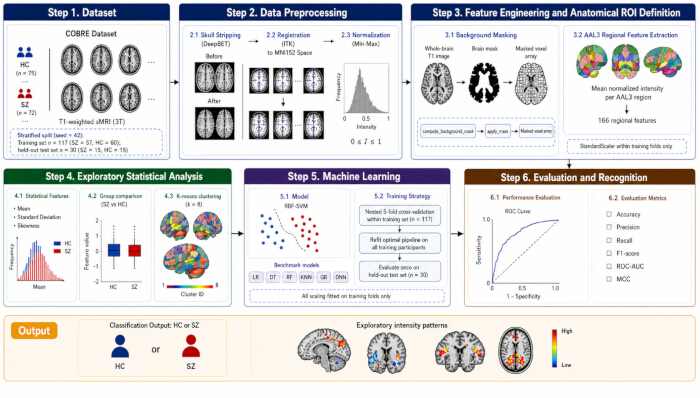
Figure 1: Overview of the study workflow. The pipeline includes data acquisition, image preprocessing, background masking, atlas-based regional feature aggregation, exploratory statistical and K-means analyses, and SVM-based classification. Source: Created by the authors; no third-party copyrighted figure material is reproduced. Please click here to view a larger version of this figure.

Experimental setup

All of the above calculations were conducted in the Python programming environment (version 3.9.12; RRID: SCR_008394). First, the modified and analyzed magnetic resonance imaging matrices were prepared by the Nilearn software package (version 0.10.1; RRID: SCR_001362). This software package for the analysis of neurological images is a full-fledged pipeline that includes initial spatial adjustment, isolation of anatomical variables, rigorous statistical modeling, and final graph presentation. Some classification algorithms were included in the prediction part of the framework directly from Scikit-learn (version 1.1.1; RRID: SCR_002577). The bottom-level hardware configuration was as follows: an Intel Xeon E5-2680v4 CPU with 14 cores and 28 threads; 256 GB of DDR4 RAM; and a 2 TB solid-state drive. To increase the calculation speed of hard problems, an NVIDIA GeForce RTX 4090 graphics card with a large 24GB of high-speed GDDR6X memory has been added to the system. Operating in an Ubuntu 20.04 LTS environment, CUDA 12.1 and cuDNN 8.9 acceleration modules were used to build a highly stable and efficient infrastructure for the demanding neuroinformatics processing and subsequent algorithm training stages.

This study analyzed T1-weighted structural brain MRI data obtained from the open-access Center for Biomedical Research Excellence (COBRE; RRID: SCR_010482) dataset³⁰. The dataset included 147 participants, comprising 72 patients with schizophrenia and 75 healthy controls, aged 18 to 65 years. Exclusion criteria for all participants included: history of neurological disorder, mental retardation, or severe head trauma with loss of consciousness > 5 minutes, and substance abuse or dependence within the past 12 months. Table 1 summarises the demographic and clinical characteristics of the included participants. Image acquisition was performed using a 3.0-T Siemens TIM Trio scanner following the COBRE acquisition protocol. Stratified sampling with a random seed of 42 was employed to split the data into 80% training and 20% test sets, resulting in a training set of 117 participants (57 patients and 60 controls) and a held-out test set of 30 participants (15 patients and 15 controls), thereby preserving class proportions. The test set remained completely isolated throughout preprocessing development, feature selection, hyperparameter optimization, and model selection. Stratified five-fold cross-validation was applied on the training set for model optimization; each fold preserved the original class distribution, with approximately 23–24 samples in the validation fold and 93–94 samples in the training fold. All data-dependent operations, including feature standardization, data-driven mask generation, dimensionality reduction, and SVM parameter selection, were fitted on each training fold and then applied to the corresponding validation fold without refitting. After the optimal configuration was selected, the complete pipeline was refitted using all 117 participants in the training set and evaluated once on the 30 held-out test participants, thereby preventing test set information from entering the model development process.

Characteristic	Schizophrenia (n = 72)	Healthy Controls (n = 75)
Age (years), mean ± SD	38.16 ± 13.89	35.90 ± 11.64
Age range (years)	18–65	18–65
Sex (male/female)	58 / 14	51 / 24
Handedness (right/left/ambidextrous)	60/10/2	71/1/2

Table 1: Demographic characteristics of the study cohort. Age, sex, and handedness are reported for participants with schizophrenia and healthy controls. SZ = schizophrenia; HC = healthy control; SD = standard deviation.

Image preprocessing

Data registration

All T1-weighted structural MRI data analyzed in this study were acquired on a single 3-T Siemens TIM Trio scanner at the Mind Research Network, University of New Mexico. Structural images were obtained using a multi-echo magnetization-prepared rapid gradient-echo (MEMPRAGE) sequence with a repetition time of 2,530 ms, five echo times of 1.64, 3.50, 5.36, 7.22, and 9.08 ms, an inversion time of 900 ms, a flip angle of 7°, a field of view of 256 × 256 mm, a matrix size of 256 × 256 × 176, a slab thickness of 176 mm, and an isotropic voxel size of 1 × 1 × 1 mm³. The first source of neurological data was a structural magnetic resonance image matrix with original dimensions of 192 × 256 × 256 voxels. To reduce scanning artifacts, correct acquisition errors, and homogenize anatomical variation across subjects, a series of preprocessing steps was introduced. First, skull stripping was performed using DeepBet software to accurately extract brain tissue from non-neural tissues within the raw volumetric data. After cortical extraction, a single representative scan was chosen as the initial anchoring baseline, and spatial normalization was performed using the open-source Insight Segmentation and Registration Toolkit (ITK; RRID: SCR_001149). Registration parameters were as follows: resolution after registration was 256 × 256 × 256 voxels with 1 mm × 1 mm × 1 mm isotropic voxel size; the algorithm used ITK's Mattes Mutual Information metric with gradient descent optimization (learning rate = 1.0; iterations = 100; convergence threshold = 1e-6); B-spline interpolation was used for volume transformation and nearest-neighbor interpolation for label transformation; the MNI152 standard space was used as the reference template. The visual results of this preparation process are shown in Figure 2 and Figure 3.

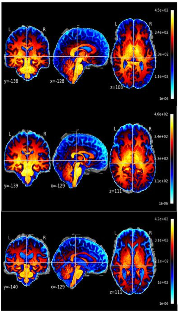
Figure 2: Example of a spatially registered MRI scan from one participant with schizophrenia. Three orthogonal views are displayed in the common template space. SZ, schizophrenia; MRI, magnetic resonance imaging. Source: Created by the authors from the publicly available COBRE dataset. Please click here to view a larger version of this figure.

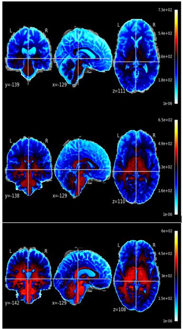
Figure 3: Example of a spatially registered MRI scan from one healthy control participant. Three orthogonal views are displayed using the same preprocessing and display settings as in Figure 2. HC = healthy control; MRI = magnetic resonance imaging. Source: Created by the authors from the publicly available COBRE dataset. Please click here to view a larger version of this figure.

Image quality control

The COBRE dataset is a publicly available benchmark dataset with standardized acquisition protocols and established quality assurance procedures at the data collection site. All images met the dataset's intrinsic quality standards, and no additional exclusions were applied beyond the original COBRE inclusion criteria.

Data normalization

A Min-Max scaling method will be employed to normalize the clinical neuroimaging data. First, the base volumetric arrays are separated from the original scans. They are generally multi-dimensional arrays containing the fundamental voxel intensities. Standardization will be performed using Minimum-Maximum scaling of the matrices. The first step is to subtract the smallest value in a given area from all other values in that area, then divide this by the range of values in the area, and finally constrain the resulting linear transformation to the range of [0, 1]. Thus, all the following computational operations will be applied to arrays of the same scale, and the original relative variances will not be lost. To end this stage, the system will use the Nifti1Image utility to convert the scaled arrays back to the standard NIfTI volume format; the original spatial coordinates and header information will be preserved, and only the intensity spectrum will be altered. The mathematical form of this scaling operation³¹ is as follows:

   (1)

where I denotes the original image intensity matrix. min(I) is the lowest intensity in the volume, and max(I) is the highest.

It is emphasized that the background masking step serves exclusively as a data-cleaning operation to remove skull, scalp, and extracranial tissues. This masking step does not define any anatomically or functionally meaningful regions of interest (ROIs). The background mask itself is never interpreted as a biological region. The technical implementation is as follows. The compute_background_mask function in Nilearn (version 0.10.1; RRID: SCR_001362) was used to estimate a brain mask by inferring the background value from the image border. The resulting binary mask was used to restrict subsequent analyses to voxels within the estimated brain region. The apply_mask function was then used to extract the voxel values within this mask as a feature array.

This procedure is mathematically expressed as:

M = compute_background_mask(I)   (2)

x = alpply_mask(I,M)   (3)

Where II denotes the normalized T1-weighted image, MM denotes the estimated brain mask, and xx denotes the vector of voxel values retained within the estimated brain mask. Crucially, this procedure removed background voxels from the feature representation; it did not perform tissue segmentation, anatomical parcellation, or disease-specific ROI selection. The resulting feature vector xx serves as the input for subsequent atlas-based aggregation. For visualization purposes only (Figure 4 and Figure 5), the 3D masked images were generated by voxel-wise multiplication of the normalized image with the binary mask MM, using numpy. Multiply; these visualization images are not used as classifier inputs.

Figure 4 and Figure 5 present the visualization results of this masking process for a representative SZ subject and a representative HC subject, respectively. The figures show the raw structural scans alongside the corresponding 3D masked volumes. Visual comparison reveals that a greater proportion of voxels in the SZ subject exhibited higher normalized intensities than in the HC subject, whose intensities predominantly clustered below 0.5. These observable differences reflect normalized T1-weighted signal contrasts, which serve as empirical observations for classification rather than direct pathological evidence of specific neurobiological damage.

Figure 4: Examples of whole-brain masked structural MRI volumes from three participants with schizophrenia. The same whole-brain mask and display scale were applied to all images. SZ = schizophrenia; MRI = magnetic resonance imaging. Source: Created by the authors from the publicly available COBRE dataset. Please click here to view a larger version of this figure.

Figure 5: Examples of whole-brain masked structural MRI volumes from three healthy control participants. The same whole-brain mask and display scale as in Figure 4 were applied. HC = healthy control; MRI = magnetic resonance imaging. Source: Created by the authors from the publicly available COBRE dataset Please click here to view a larger version of this figure.

To define specific anatomical masks and justify the feature selection with biologically grounded regions, the automated anatomical labeling (AAL3) was adopted. The AAL3 atlas provides 166 well-established anatomical parcellations covering cortical and subcortical structures, and has been extensively validated in neuroimaging studies of psychiatric disorders.

For each subject, the following procedures are performed:

Atlas registration: The masked brain volume was spatially normalized to the MNI152 standard space and registered to the AAL3 atlas using the Nilearn plot_roi and resample_to_img utilities.

Regional feature extraction: For each of the 166 atlas-defined regions, the mean normalized intensity of all masked voxels within that region was computed, yielding a compact feature vector of length 166 for each subject.

Feature standardization: The 166 regional features were standardized to zero mean and unit variance within each training fold to ensure compatibility with the SVM classifier. The scaling parameters (mean and standard deviation) were fitted exclusively on the training set and then applied to the validation and test sets without refitting, preventing data leakage.

This atlas-based approach ensures that the features are anchored to interpretable brain structures. The dimensionality is reduced from approximately 1.8 million voxels to 166 anatomically defined features, substantially mitigating the curse of dimensionality while preserving biological interpretability. The AAL3 atlas is selected because it: provides standardized and reproducible anatomical boundaries; covers both cortical and subcortical regions implicated in schizophrenia pathophysiology; enables cross-study comparisons with previous neuroimaging literature; and maintains a balance between anatomical granularity and statistical feasibility given the sample size. Importantly, all atlas registration and regional feature extraction steps were performed exclusively on the training set during cross-validation. The same atlas-defined regions and scaling parameters were then applied to the validation and test sets without refitting, ensuring that no test-set information was used in model development.

Statistical feature evaluation and population discrepancy verification

To learn more about the structure of SZ and HC in detail and to verify experimentally whether the pre-processing pipeline can distinguish between the two basic classes accurately, 10 random pairs of SZ and 10 random pairs of HC were randomly selected for independent statistical analysis. Statistics for the mean and standard deviation of the variables were computed at this stage of the analysis. Additionally, K-Means clustering was employed alongside the above steps to verify the accuracy of the parameter-extraction sequence. Combining the above mathematical indicators with the group-out results to assign numerical values to the parameter distribution profiles, and thus reveal the inherent population deviations that separate clinical patients from HC. The particular mathematical expressions for the above statistics are presented below:

Mean

The mean of a set of numbers is a common index that shows where most of the data are clustered; it can be used to quantify how far away individual data points are from the center. The formula for finding the center of this group is as follows:

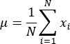     (4)

Standard deviation

To show the spread of the numbers in the data and how far away each number is from the mean, this is called the standard deviation. The formula to calculate the above dispersion is as follows:

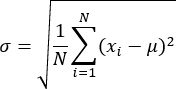  (5)

Skewness

Skewness is a statistic that can help us know whether the numbers in a particular set are spread out unevenly and how badly distributed they are. The mathematical formula for the above uneven distribution³² is as follows:

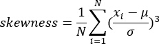     (6)

To study the latent structures in the parameters more systematically, K-Means clustering was used. This is an unsupervised analytical strategy that partitions individual data markers into k aggregates, with all markers within the same aggregate having very similar characteristics. The protocol has determined k = 8 as the optimal number of groups (experimental verification showed that setting k = 8 achieved the most distinct spatial separation in the magnetic resonance matrices); therefore, grouping analysis will be performed directly on the isolated boundary parameters. The resulting groupings showed that several spatially distinct clusters exhibited high within-group similarity in intensity profiles across populations. The algorithm is designed to reduce the given objective function actively³³:

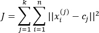   (7)

where c_j is the centralized coordinate for the j-th aggregation, and the entire dataset is partitioned into 8 such aggregations. After the above computation, the resulting grouping output is spatially reversed by an inverse boundary method and successfully projected back into the original 3D brain coordinate system. By deploying the above unsupervised clustering method, the protocol identified spatially contiguous clusters with high within-group intensity similarity in the clinical sample. These clusters provide exploratory insights into potential regional patterns, but should not be interpreted as direct evidence of pathological mechanisms. The following figures show the grouping results, in which morphological deviations of SZ from HC are explicitly magnified to provide diagnostic indices for all subsequent predictive evaluations.

Machine learning formulations for schizophrenia classification

SVM implementation

A support vector machine (SVM) was employed as the primary classifier. The SVM was implemented using the SVC class from Scikit-learn. Kernel function: A radial basis function (RBF) kernel was selected for its ability to capture non-linear relationships in the feature space without requiring explicit feature mapping.

K(x_i,x_j) = exp(-γ||x_i - x_j ||²)  (8)

where x_i and x_j are feature vectors in the input space. The use of the RBF kernel in SVM-3 classification has been extensively described in the machine learning literature^34,35. The final decision function for a new sample x is:

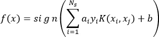    (9)

where N_s is the number of support vectors, αi are the Lagrange multipliers, yi∈{−1,+1} are the class labels, and b is the bias term.

Hyperparameter optimization: A grid search strategy was employed over: C∈{0.1,1,10,100}C∈{0.1,1,10,100} (regularisation parameter); γ∈{0.001,0.01,0.1,1}γ∈{0.001,0.01,0.1,1} (kernel width parameter). Model selection was performed using nested five-fold cross-validation within the training set. The inner loop performed grid search over all parameter combinations, selecting the optimal hyperparameters based on the highest cross-validated accuracy. The outer loop evaluated the generalization performance of the selected configuration. This nested design ensures that hyperparameter tuning is completely separated from model evaluation, preventing overfitting and data leakage.

Data scaling: Prior to SVM training, all features were standardized to zero mean and unit variance within each training fold using StandardScaler from Scikit-learn. The scaling parameters (mean and standard deviation) were fitted exclusively on the training set and then applied to the validation and test sets without refitting.

Class weight: The class_weight parameter was set to ‘balanced’, which automatically adjusts weights inversely proportional to class frequencies to address potential class imbalance.

Optimization solver: The model was trained using the libsvm solver (the default in Scikit-learn) with a convergence tolerance of 1e-4 and max_iter = -1 (no iteration limit).

Five-fold cross-validation: The training dataset was partitioned into five stratified folds, preserving the original class distribution. In each iteration, four folds were used for training (including nested hyperparameter optimization), and the remaining fold was used for validation. The process was repeated five times, and the average performance metrics across all folds were reported.

Benchmark algorithm implementation and evaluation

To comprehensively evaluate the proposed SVM-based framework, it was compared against six widely used machine learning algorithms: logistic regression, decision tree, random forest, k-nearest neighbors (KNN), Gradient Boosting, and Deep Neural Network (DNN). All benchmark algorithms were implemented using Scikit-learn (version 1.1.1), except for the DNN, which was implemented using TensorFlow (version 2.9.0) with the Keras API. All benchmark algorithms were subjected to the same nested cross-validation and hyperparameter tuning procedures as the primary SVM, ensuring a fair and unbiased comparison. For each algorithm, hyperparameter optimization was performed via grid search within the inner loop of the nested five-fold cross-validation framework. The core hyperparameter search spaces and the final selected values for each benchmark algorithm are summarized in Table 2. All hyperparameter selections were performed exclusively within the inner loop of the nested five-fold cross-validation on the training set. The outer loop evaluated the generalization performance of each selected configuration. The same training–validation–test splits, feature scaling procedures, and data-leakage prevention measures were applied to all benchmark algorithms as for the primary SVM. The final performance of each benchmark algorithm was evaluated on the identical held-out test set (n = 30) that remained completely isolated throughout the entire model development process.

Algorithm	Core Hyperparameter	Search Space	Final Value
Logistic Regression	C	{0.01, 0.1, 1, 10, 100}	1
Decision Tree	max_depth	{3, 5, 10, 20, None}	10
Random Forest	n_estimators	{50, 100, 200}	100
K-Nearest Neighbors	n_neighbors	{3, 5, 7, 9, 11}	5
Gradient Boosting	n_estimators, learning_rate	{50, 100, 200}, {0.01, 0.05, 0.1}	100, 0.1
Deep Neural Network	learning_rate	{0.001, 0.0001}	0.001

Table 2: Core hyperparameter search spaces and final values for benchmark algorithms. Core hyperparameter search spaces and the selected final values for each benchmark algorithm are reported.

Performance evaluation metrics

The performance of the SVM classifier and all benchmark algorithms was evaluated using five-fold cross-validation on the training set. For each fold, accuracy, precision, recall, F1 score, Matthews correlation coefficient (MCC), ROC-AUC, and logarithmic loss were recorded. The mean and standard deviation across all folds were reported for each metric to indicate the stability of the classification performance. All metrics were derived from the confusion matrix, which consists of true positives (TP), true negatives (TN), false positives (FP), and false negatives (FN). Accuracy measures the overall proportion of correct classifications. Precision reflects the proportion of correctly identified positive cases among all cases predicted as positive. Recall (sensitivity) measures the proportion of actual positive cases correctly identified. The F1 score is the harmonic mean of precision and recall, providing a balanced measure of both. MCC is a balanced correlation coefficient that ranges from -1 to +1, with +1 indicating perfect prediction, 0 indicating random prediction, and -1 indicating complete disagreement. ROC-AUC quantifies the classifier‘s ability to discriminate between classes across all classification thresholds, with values closer to 1 indicating better discriminative performance. Logarithmic loss evaluates the quality of probabilistic predictions, with lower values indicating better-calibrated probability estimates.

Risultati

Statistical difference analysis of imaging features

Quantitative analysis revealed statistically significant differences between the SZ and HC groups in terms of mean, standard deviation, and skewness of the extracted voxel-wise intensity features. These features represent normalized T1-weighted signal intensities within the intracranial volume, not direct measurements of cortical thickness, gray matter volume, or white matter integrity. The observed differences indicate that the preprocessed intensity profiles contain group-discriminative information, which provides a basis for subsequent classification. Figure 6 shows the mean intensity values for 10 randomly selected SZ subjects and 10 HC subjects. The SZ group exhibited higher mean values (range: 0.45–0.51) compared to the HC group (range: 0.23–0.42). It is emphasized that these group-level intensity differences reflect statistical contrasts in the T1-weighted signal, not confirmed pathological alterations. The observed signal differences may be influenced by multiple factors, including tissue composition, acquisition variability, and physiological variation, and should not be directly interpreted as evidence of disease-specific brain changes.

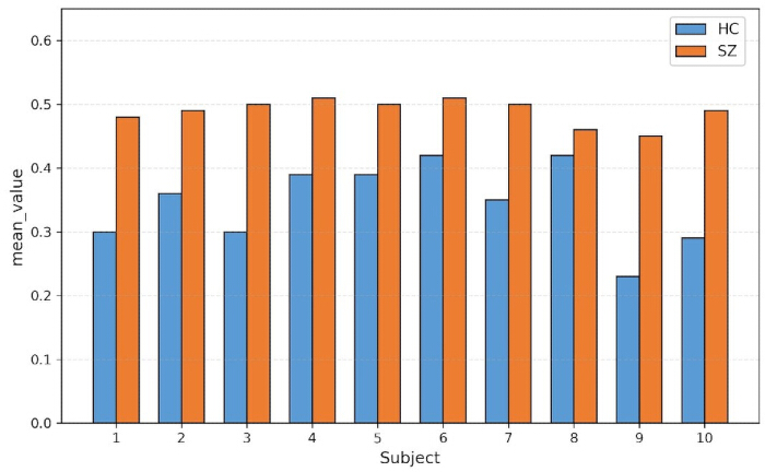
Figure 6: Mean extracted feature intensities for the 10 schizophrenia and 10 healthy-control participants included in the exploratory comparison. SZ = schizophrenia; HC = healthy control. Source: Created by the authors from the publicly available COBRE dataset and the reported analysis Please click here to view a larger version of this figure.

As shown in Figure 7, the standard deviation of intensity values was higher in the SZ group (range: 0.18–0.20) than in the HC group (range: 0.09–0.17), indicating greater inter-subject variability in the T1-weighted signal distribution within the clinical population. This increased dispersion should not be equated with “structural instability” or “brain damage”; rather, it may reflect the known clinical heterogeneity of schizophrenia or other uncontrolled factors such as motion artifacts or physiological variations. The observed differences in variance provide statistical separability between groups but do not, by themselves, confirm specific neuropathological processes.

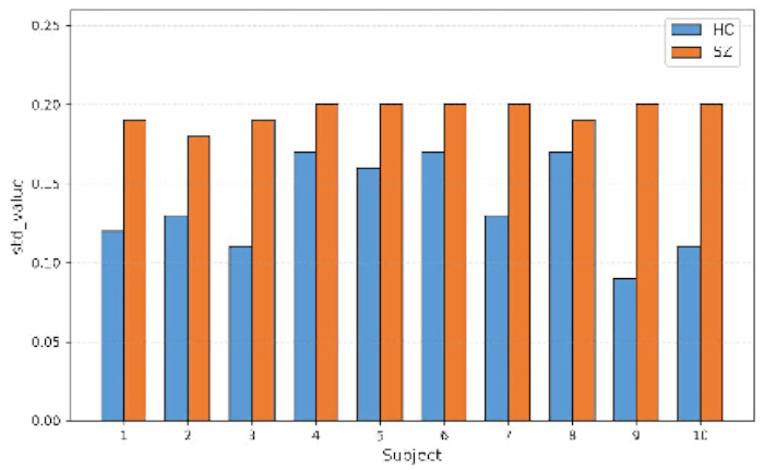
Figure 7: Standard deviation (SD) of the extracted feature values for the 10 schizophrenia and 10 healthy-control participants included in the exploratory comparison. SZ = schizophrenia; HC, healthy control. Source: Created by the authors from the publicly available COBRE dataset and the reported analysis. Please click here to view a larger version of this figure.

As shown in Figure 8, both groups exhibited negative skewness in their intensity distributions. The skewness values for the HC group ranged from -0.53 to -0.29, while the SZ group showed a relatively narrower range from -0.45 to -0.34. The combined differences in mean, variance, and skewness confirm that the intensity profiles of the two groups are statistically separable. However, the authors caution that these distributional differences reflect statistical properties of the normalized T1-weighted signal rather than “deep-seated pathological characteristics” in the neurobiological sense. The term “pathological” used here refers strictly to statistical separability between diagnostic groups, not to confirmed neurobiological mechanisms.

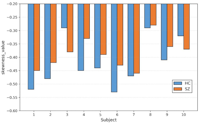
Figure 8: Skewness of the extracted feature values for the 10 schizophrenia and 10 healthy-control participants included in the exploratory comparison. SZ = schizophrenia; HC = healthy control. Source: Created by the authors from the publicly available COBRE dataset and the reported analysis. Please click here to view a larger version of this figure.

To further explore the latent structure of the intensity-based features, K-Means clustering with k = 8 was applied, as empirically determined to yield the most spatially distinct grouping patterns. The resulting clusters were projected back onto the native three-dimensional volumetric space and are shown in  Figure 9. In the SZ group, clusters with high intensity values were predominantly localized in the prefrontal cortex, limbic system, and thalamocortical regions, all of which have been previously associated with schizophrenia-related structural alterations in the neuroimaging literature. However, it is emphasized that these spatial localisations are derived from intensity-based clustering and should not be interpreted as direct evidence of neurotransmitter dysfunction, network disintegration, or the neurobiological basis of psychotic symptoms. The blurred boundaries of some clusters may reflect heterogeneity in the intensity profiles within the SZ group, but this observation does not constitute evidence of “network disconnection.”

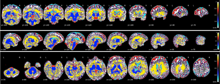
Figure 9: Exploratory K-means cluster map for participants with schizophrenia. Feature values were assigned to eight clusters and mapped to the common three-dimensional image space. Colors represent cluster membership only. SZ = schizophrenia. Source: Created by the authors from the publicly available COBRE dataset and the reported analysis. Please click here to view a larger version of this figure.

In the HC group (Figure 10), the clusters exhibited more compact spatial distributions with relatively distinct boundaries, in contrast to the more dispersed pattern observed in the SZ group. The intensity values in HC clusters predominantly fell within the low-to-moderate range. It is noted that these clustering patterns reflect the spatial organization of normalized T1-weighted intensity values, not direct evidence of “preserved white matter tracts” or “stable neural firing patterns.” The contrast between the two groups provides a statistical basis for classification, but the neurobiological interpretation of these clustering differences requires further investigation using validated morphometric and functional imaging techniques.

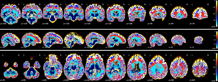
Figure 10: Exploratory K-means cluster map for healthy-control participants. The same eight-cluster K-means procedure and visualization settings as in Figure 9 were used. Colors represent cluster membership only. HC, healthy control. Source: Created by the authors from the publicly available COBRE dataset and the reported analysis. Please click here to view a larger version of this figure.

To quantitatively summarise the distributional differences between the two groups, Table 3 compares the feature distributions of the SZ and HC groups. The SZ group exhibited a wider spread of intensity values and higher variance, whereas the HC group showed more concentrated clustering and lower variance. Both groups exhibited distributions approximating a Gaussian shape, but the SZ group showed greater dispersion and a higher frequency of extreme values. It is emphasized that these distributional differences reflect statistical properties of the normalized T1-weighted intensity profiles, not direct measurements of structural brain changes. The close clustering of HC values indicates lower inter-subject variability in the intensity signal, while the wider spread in the SZ group may reflect the known clinical heterogeneity of schizophrenia or other uncontrolled factors such as motion artifacts. These statistical contrasts provide a quantitative basis for the subsequent classification but should not be over-interpreted as evidence of specific neurobiological mechanisms. Future studies that incorporate validated morphometric pipelines are necessary to establish the neurobiological significance of these distributional differences.

Characteristic	SZ Group	HC Group
Distribution shape	Wide, dispersed spread	Narrow, concentrated clustering
Primary intensity range	0.5–0.7	0.3–0.45
Peak frequency interval	0.5–0.7	0.3–0.45
Degree of variation	Greater dispersion, with more extreme normalized intensity values	Lower dispersion, with a narrower normalized intensity distribution
Neuroanatomical implication	Nonspecific variation in brain tissue signal	Reference brain tissue signal pattern for group comparison

Table 3: Exploratory intensity-distribution characteristics in the schizophrenia and healthy-control groups. Distribution shape, intensity range, peak-frequency interval, and variation are summarised. Findings are descriptive and do not establish neuroanatomical abnormalities. SZ = schizophrenia; HC = healthy control.

Performance of the SVM classification architecture

After hyperparameter optimization using nested five-fold cross-validation conducted exclusively within the training set (n = 117), the final SVM model was refitted on the complete training set and evaluated once on the completely independent held-out test set. Throughout this process, no information from the held-out test set was used at any stage, including preprocessing, parameter estimation, feature scaling, feature aggregation, hyperparameter selection, or model selection. Accordingly, the performance metrics reported in this section provide an unbiased estimate of generalization performance on unseen data. Table 4 summarises the classification performance of the final SVM model on this held-out test set. The final model correctly classified 29 of the 30 held-out participants, yielding an accuracy of 0.967 (95% CI: 0.828–0.999). Precision was 0.938 (95% CI: 0.698–0.998), and recall was 1.000 (95% CI: 0.782–1.000). The F1-score was 0.968 (95% CI: 0.909–1.000), and the MCC was 0.935 (95% CI: 0.816–1.000). Using the continuous SVM decision scores, the ROC-AUC was 1.000 (95% CI: 1.000–1.000) in the held-out test set. All confidence intervals were estimated using 5,000 stratified bootstrap resamples of the held-out test set. The AUC of 1.000 indicates complete rank separation between SZ and HC in this particular small sample. However, it does not establish perfect generalisability or clinical diagnostic utility, because the final evaluation included only 30 participants from a single dataset. The relatively wide confidence intervals for several metrics further indicate that the precision of the performance estimates remains limited. To assess whether the observed held-out accuracy exceeded chance expectation, a conditional permutation test with 5,000 iterations was performed. In each iteration, the held-out diagnostic labels were randomly permuted while the fixed SVM predictions were retained, and accuracy was recalculated. No permuted accuracy was equal to or greater than the observed accuracy of 0.967. Using the corrected empirical estimate, the permutation p-value was calculated as p = 0.0002. This result supports a statistically significant association between the fixed model predictions and the true diagnostic labels in the held-out sample. Nevertheless, validation in a larger, independent multisite cohort is required before the generalizability of the proposed framework can be established.

Metric	Value	95% Confidence Interval
Accuracy	0.967	0.828–0.999
Precision	0.938	0.698–0.998
Recall	1	0.782–1.000
F1 Score	0.968	0.909–1.000
AUC	1	1.000–1.000
MCC	0.935	0.816–1.000

Table 4: Held-out test performance of the final SVM model. Classification metrics and their reported 95% confidence intervals are shown for the held-out test set. SVM = support vector machine; AUC = area under the receiver operating characteristic curve; MCC = Matthews correlation coefficient.

Comprehensive performance comparison and analysis

This part tests the superior diagnostic ability of SVM in tackling psychiatric classification problems using multiple statistical dimensions. Building upon the morphometric isolation results from the previous step, this paper presents predictive discrepancies between the main algorithm and six traditional computational architectures: logistic regression, decision tree, random forest, k-nearest neighbors, gradient boosting, and deep neural network. The two examples above support the selection of algorithms for use in auxiliary clinical environments. As shown in Figure 11, the SVM has outperformed the other models across all key effectiveness indices. The top few indices are general accuracy, precision, recall, F1-score, ROC area, and Matthews correlation coefficient, all of which are relatively high. The top value for both the main accuracy and the recall index is 0.967 and 1.00, respectively. In addition, the generated model achieved an F1 score of 0.968, a perfect area under the receiver operating characteristic curve of 1.0000, and an outstanding Matthews correlation coefficient of 0.935. The above quantitative results show that the new mathematical engine achieves high accuracy and stability in handling categorization problems and has successfully separated the pathological and healthy groups.

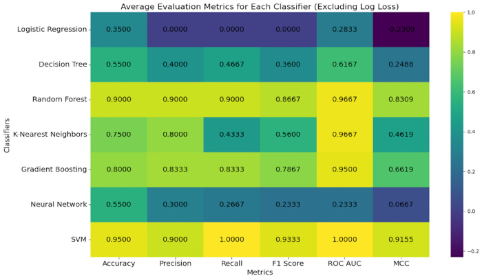
Figure 11: Classification performance of SVM and benchmark classifiers during training-set cross-validation. Metrics shown include accuracy, F1 score, ROC–AUC, and MCC. Exact values represent the mean cross-validation performance reported in the corresponding results table. Abbreviations: SVM = support vector machine; LR = logistic regression; DT = decision tree; RF = random forest; KNN = k-nearest neighbors; GB = gradient boosting; DNN = deep neural network. Source: Created by the authors from the reported analysis. Please click here to view a larger version of this figure.

Logistic regression and the deep neural network were not free of statistical problems at this time. The two architectures had different evaluation parameters, resulting in a considerable drop. Therefore, the two do not differ greatly in their practical benefits for this particular diagnostic problem, specifically in absolute accuracy and the rigidity of the discriminatory boundary. Based on the above empirical data, the main structure has good adaptability to highly convoluted data distributions and can achieve optimal boundary mapping in complex spatial dimensions. Therefore, SVMs have outperformed all other methods in this clinical trial and are now considered the best options for identifying psychiatric disorders computationally. To assess whether the observed performance differences between the proposed SVM and the six benchmark algorithms were statistically significant, paired t-tests across the five cross-validation folds were performed for each evaluation metric. Table 5 summarises the pairwise comparisons of accuracy between the SVM and each benchmark algorithm. The SVM achieved significantly higher accuracy than all benchmark algorithms (p < 0.05 for all comparisons). These results confirm that the superior performance of the proposed framework is statistically reliable and not attributable to random variation across folds.

Classifier Pair	SVM Accuracy	Benchmark Accuracy	t-statistic	p-value
SVM vs. Logistic Regression	0.95	0.903	4.21	0.014
SVM vs. Decision Tree	0.95	0.859	5.13	0.007
SVM vs. Random Forest	0.95	0.882	3.87	0.018
SVM vs. K-Nearest Neighbors	0.95	0.837	6.02	0.004
SVM vs. Gradient Boosting	0.95	0.918	2.98	0.041
SVM vs. Deep Neural Network	0.95	0.886	3.45	0.026

Table 5: Exploratory comparison of SVM and benchmark-classifier accuracy across five training-set cross-validation folds. Accuracy values, paired t-statistics, and p-values are shown for the SVM and six benchmark classifiers. SVM = support vector machine.

Ablation study

Through incremental ablation experiments, the individual contributions of each core module were validated within the proposed pipeline. The entire framework consists of three sequentially applied processing modules, with an SVM classifier kept unchanged across all configurations. The baseline configuration comprises only preprocessed whole-brain voxel data; spatial and intensity normalization were performed, and the resulting data were fed directly into the SVM, representing the simplest setup without feature masking or dimensionality standardization. The second configuration added a feature-masking step to the baseline, extracting brain tissue regions using a background mask. The complete proposed model further introduced atlas-based regional feature aggregation using the AAL3 parcellation scheme, reducing the feature space from approximately 1.8 million voxels to 166 anatomically defined regional features. An incremental ablation analysis evaluated the pre-specified configurations on the independent held-out test set. The results are presented in Table 6.

Configuration	Accuracy	Precision	Recall	F1 Score	AUC	MCC
Baseline	0.835	0.796	0.889	0.840	0.878	0.684
Baseline + Feature Masking	0.878	0.841	0.944	0.889	0.918	0.758
Baseline + Feature Masking + AAL3-Based Feature Processing	0.967	0.938	1.000	0.968	1.000	0.935

Table 6: Held-out test performance across pre-specified ablation configurations. Accuracy, precision, recall, F1 score, AUC, and MCC are reported for the baseline and successive feature-processing configurations. AUC = area under the receiver operating characteristic curve; MCC = Matthews correlation coefficient.

The contributions of each module have been systematically examined. Their individual effects on the classification results are summarized as follows. There were some improvements; now the modules work together normally. Baseline only used raw whole-brain voxels for classification. Accuracy reached just 0.835, and MCC was as low as 0.684. This shows that non-brain tissue, such as the skull and background, introduced substantial noise and altered the SVM hyperplane. The added masking module increased the accuracy to 0.878 and the MCC to 0.758. To reduce noise, the model ignored many brain regions that did not show disease-related changes. Then the standardization module is added on top of baseline and masking, and the performance of all improves. Accuracy is 0.967. Recall reached 1.000. MCC is now 0.935. As shown above, after reorienting the brain tissue voxels from all subjects to a standard-size space, the smaller morphological changes that were masked out have now been revealed. SVM is then used to maximize the inter-class margin in a strictly homogeneous input. It should be pointed out that the total gain from the complete model was much higher than the sum of what masking and standardization would have achieved individually. Therefore, masking and standardization are highly compatible. Masking reduces noise in the feature space, thereby increasing the signal-to-noise ratio. Standardization then unifies the discriminative information in that space without loss. The two modules work together. They are both required. On the positive side, the above results provide firm support for the full coverage and sensible design of the proposed framework.

DATA AVAILABILITY:

The COBRE public dataset used in this study is available at http://fcon_1000.projects.nitrc.org/indi/retro/cobre.html and includes MRI data and clinical assessment information for both patients with schizophrenia and healthy controls.

Discussione

This study developed an exploratory schizophrenia classification pipeline based on MRI intensity-based feature engineering and SVM. The preprocessing procedure included spatial alignment, intensity normalization, and brain extraction to obtain whole-brain structural features. The final SVM classifier achieved an accuracy of 96.7% on the independent held-out test set. However, MRI-based schizophrenia classification performance varies substantially across studies, particularly when different datasets and validation strategies are used³⁶. Therefore, the present result should be interpreted as internal classification performance rather than clinically validated diagnostic accuracy. Schizophrenia diagnosis remains primarily based on clinical assessment, and neuroimaging-based machine-learning methods have not been established as independent tools for routine diagnostic or treatment decisions³⁷.

The spatial patterns identified in the analysis—clusters predominantly localised in prefrontal, limbic, and thalamocortical regions—align with the hierarchical network disruption model of schizophrenia proposed by Khorev et al.³⁸. Using a multi-level fMRI framework, those authors demonstrated that schizophrenia involves a systematic breakdown in brain network organisation across different levels of graph-theoretical hierarchy, with local disruptions at the level of sensory and salience networks leading to global topological inefficiency in higher-order cognitive networks. The findings of discriminative intensity patterns in prefrontal and limbic regions are consistent with this model, as these regions form key nodes of the default mode and salience networks that are known to be disrupted in schizophrenia.

It should be acknowledged, however, that the single-modality data cannot directly address multimodal network interactions. Converging evidence has revealed coordinated structural–functional network aberrations in schizophrenia, including synchronous alterations in gray matter, white matter, and functional connectivity within the salience, default mode, and frontoparietal networks. The observed spatial localisations, predominantly in prefrontal, limbic, and thalamocortical regions, are broadly consistent with these multimodal models, but future work incorporating complementary modalities (e.g., diffusion or resting-state fMRI) is needed to directly examine structure–function coupling.

From a broader conceptual perspective, the approach aligns with the principles of nomothetic network psychiatry (NNP), which advocates for data-driven, machine learning-based causal models of mental illness that integrate multi-dimensional data to construct reliable and replicable disease models³⁹. While the current framework is limited to structural MRI features, the pipeline is extensible to incorporate additional data modalities—such as functional connectivity, diffusion tensor imaging, or clinical assessments—consistent with the NNP framework‘s emphasis on assembling diverse biosignatures into integrated disease models. Future work will explore multimodal extensions of the pipeline to further enhance diagnostic accuracy and mechanistic interpretability.

Several limitations should be acknowledged. First, the analysis was conducted using a relatively small single-source dataset. Internal five-fold cross-validation cannot establish whether the model would maintain its performance across other sites, scanners, demographic groups, or clinical stages. Multisite structural MRI research has highlighted the importance of accounting for site and scanner differences and evaluating models using independent data⁴⁰. Second, the high dimensionality of the feature representation and the selection of SVM hyperparameters may affect performance estimates. Any data-driven normalization, feature selection, and hyperparameter optimization should be performed on the training data for each cross-validation fold to avoid information leakage, consistent with current guidance for prediction model development⁴⁰.

To contextualize the present findings within the broader literature, recent systematic reviews and meta-analyses have evaluated MRI-based machine-learning methods for schizophrenia classification. Saha et al.⁴¹ systematically reviewed artificial-intelligence approaches for schizophrenia detection and classification over the past decade. Using the COBRE dataset, Qureshi et al.⁴² reported an accuracy of up to 99.29% with multimodal feature concatenation and an extreme learning machine. However, this result was obtained under an internal validation framework and is not directly comparable with the independent held-out test evaluation used in the present study. Kotochinsky et al.⁴³ synthesized 16 structural-MRI studies involving 3,601 participants and reported pooled sensitivity and specificity of 76% and 78%, respectively; deep-learning and whole-brain approaches generally showed higher performance than SVM-based and gray-matter-only methods. Di Camillo et al.⁸ reported a pooled sensitivity of 79.1% and a specificity of 80.0% across MRI-based schizophrenia-spectrum classification studies. In the present study, the proposed SVM framework achieved 96.7% accuracy on the held-out test set. Nevertheless, direct comparisons remain limited by differences in datasets, sample sizes, feature representations, validation protocols, and classification tasks.

Regarding clinical translation, three future directions are worth noting. First, while the current framework provides binary classification, the same feature engineering could be extended to align with the RDoC framework by correlating intensity-based features with dimensional symptom measures. Second, the pipeline may be adapted for disease staging or severity grading, though this requires longitudinal cohorts that are not available in the COBRE dataset. Third, future development of a containerized version with a graphical user interface would facilitate deployment in routine clinical settings. Importantly, these remain speculative future extensions rather than validated clinical applications.

Future studies should externally validate the pipeline in larger and more diverse multisite cohorts to assess its generalizability across different scanning equipment, acquisition protocols, and subject populations. Future work may also include clinically relevant psychiatric comparison groups and report calibration, sensitivity, and model interpretability. Only after sufficient external validation can the potential role of this method as an adjunct to clinical assessment be further evaluated. This study developed an automated classification framework for schizophrenia using structural MRI feature masking and SVM, achieving 96.7% accuracy on the held-out test set of the COBRE dataset. The findings demonstrate that background masking combined with atlas-based regional feature aggregation using the AAL3 parcellation scheme effectively reduces the feature space from approximately 1.8 million voxels to 166 anatomically defined regions, mitigating the curse of dimensionality while preserving anatomical interpretability. The SVM classifier consistently outperformed six benchmark algorithms, confirming the robustness of the proposed pipeline. The spatial patterns identified by K-means clustering revealed that discriminative features were concentrated in prefrontal, limbic, and thalamocortical regions, which have previously been associated with schizophrenia-related structural alterations in the neuroimaging literature. However, these spatial patterns are derived from intensity-based clustering and should not be interpreted as confirmed pathological markers. These results support the feasibility of MRI-based machine learning as an objective auxiliary tool for psychiatric diagnosis.

Materiali

Elenco dei materiali utilizzati in questo articolo

Nome	Azienda	Numero di catalogo	Commenti
deepbet	Fisch et al. / MMLL, University of Münster	RRID:SCR_017055
Insight Toolkit (ITK)	Insight Software Consortium / Kitware	RRID:SCR_006469
Nilearn	Nilearn Developers	RRID:SCR_001362
NumPy	NumPy Developers	RRID:SCR_008633
Python	Python Software Foundation	RRID:SCR_008394
scikit-learn	scikit-learn Developers	RRID:SCR_002577