Depth-Mining Network with Edge-Sensitive Context for Red-Green-Blue-Depth Surface Defect Segmentation

Sommario

This study presents Depth-Mining Network with Edge-sensitive context, a red-green-blue-depth surface defect segmentation network that selectively mines reliable depth cues and incorporates edge-sensitive context to improve defect localization, boundary refinement, and cross-modal robustness.

Abstract

Red-green-blue-depth (RGB-D) surface defect segmentation combines RGB and depth information to perceive the spatial distribution of defects in complex, low-contrast scenes. Current RGB-D methods typically rely on an undifferentiated bidirectional interaction mode that treats RGB and depth information equally, making them susceptible to poor-quality depth data. To address this issue, this article introduces a Depth-Mining Network with Edge-sensitive context (DMENet), which selectively mines complementary depth information and incorporates edge context to enhance defect feature representation. During encoding, a Depth-Mining Feature Fusion (DMFF) module mines depth information that is semantically relevant to RGB features and adaptively fuses it with RGB information. During decoding, a Hierarchical Feature Aggregation (HFA) module combines RGB-D, RGB, and depth features to preserve defect information. An Edge-Guided Feature Enhancement (EGFE) module further refines defect boundaries. Experiments on the Northeastern University Rail Surface Defect Detection Dataset (Augmented version, NEU RSDDS-AUG) demonstrate that DMENet achieves a mean absolute error (MAE) of 0.0483, an S-measure of 0.867, a maximum E-measure of 0.947, and a maximum F-measure of 0.911, outperforming state-of-the-art methods. It also achieves MAE values of 0.017, 0.026, and 0.032 on the National Laboratory of Pattern Recognition (NLPR), Nanjing University 2K (NJU2K), and STEREoscopic (STERE) datasets, respectively. Robustness was further demonstrated across three random seeds (MAE = 0.0483 ± 0.0004), 16 input perturbation settings, and the industrial NEU-Seg steel surface defect dataset (MAE = 0.1111), indicating stable performance and cross-material generalization in industrial settings.

Introduzione

Surface defect detection plays a crucial role in industrial manufacturing and product maintenance. Deep learning-based surface defect detection networks can identify defects across different levels, including image-level^1,2,3, region-level^4,5,6, and pixel-level^7,8,9, making quality control in industrial production more reliable and efficient. Current surface defect detection methods primarily rely on a single RGB or grayscale modality, which struggles to distinguish defects that have colors and textures similar to the background.

With advancements in depth imaging technology, depth images have been integrated into defect detection networks^10,11,12,13 to improve performance by providing explicit geometric structure information, particularly for defects under cluttered background noise in a single modality. Current red-green-blue-depth (RGB-D) defect detection methods^14,15, which are primarily based on the undifferentiated bidirectional interaction mode, treat depth and RGB information equally but face two main issues. First, in defect scenes with weak spatial cues, minimal depth differences between foreground and background hinder depth perception. Second, RGB and depth images contain different information, as RGB data focuses on color, texture, and brightness, while depth data emphasizes spatial structure, making semantic alignment challenging. These limitations make such methods susceptible to depth quality and less effective at exploiting complementary information in surface defect detection. As shown in Figure 1, PICRNet¹⁶ and the proposed method can utilize depth information to improve the detection performance. When depth information is poor, PICRNet's performance is noticeably degraded, even compared to DMENet on the single RGB modality.

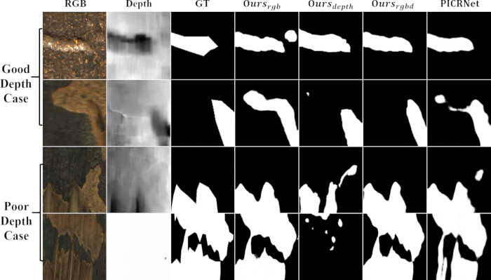
Figure 1: Comparison of prediction maps generated from DMENet in different modalities and PICRNet. Qualitative results across good-depth and poor-depth cases comparing input RGB images, depth maps, ground truth masks, single-modality predictions (Ours_rgb, Ours_depth), full RGB-D predictions (Ours_rgbd), and predictions from PICRNet. Abbreviations: RGB = Red-Green-Blue; D = Depth; GT = Ground Truth; DMENet = Depth-Mining Network with Edge-Sensitive Context; PICRNet = Point-Aware Interaction and CNN-Induced Refinement Network. Please click here to view a larger version of this figure.

In addition, defects typically exhibit irregular, indistinct contours, which degrade detection performance. Edge-prior methods can mitigate this issue by enabling the network to refine boundaries. Since depth images provide intuitive spatial structure, some RGB-D surface defect detection methods^11,17 typically use shallow depth features to extract edge information. However, these features often struggle to provide reliable details in low-contrast defect scenes, leading to poor edge information and compromised detection performance. Furthermore, simplistic boundary-refinement designs fail to fully and effectively exploit multi-level edge-related features across modalities, limiting their ability to address complex defect patterns.

To address these issues, this article proposes a Depth-Mining Network with Edge-sensitive context (DMENet) for surface defect segmentation. DMENet mines valuable depth information that can be semantically aligned with RGB features. By leveraging valuable depth information to assist RGB features, DMENet obtains enriched and robust feature representations for defects. Meanwhile, it leverages the characteristics and complementary information of modalities at different levels, incorporating edge information to refine boundaries at both coarse and fine granularities.

In DMENet, a Depth-Mining Feature Fusion (DMFF) module is introduced during the encoding stage to capture critical visual information shared across modalities. It enhances the richness of feature representation while suppressing redundant information to obtain valid RGB-D features. The DMFF module first leverages RGB features to guide depth features, thereby appropriately calibrating depth information at the pixel level. Subsequently, it aligns RGB and depth features at the channel level, ensuring that their semantics are complementary to achieve sufficient and robust cross-modal interaction. To focus on defect-related regions, the Synergistic Spatial Attention (SSA) module is proposed to concentrate on mutually salient spatial regions across modalities. In the decoding stage, a Hierarchical Feature Aggregation (HFA) module is designed to smooth the sampling process and aggregate defect details across different levels and modalities.

Furthermore, to refine the defect boundaries, a Context-Aware Edge Detector (CAED) and an Edge-Guided Feature Enhancement (EGFE) module are designed. CAED balances defect texture details and semantic information by combining specific low-level and high-level features from different modalities, thereby generating contextual, edge-sensitive defect features during edge map learning. The EGFE module incorporates edge information from the CAED into the decoding features, using the combination of coarse and fine granularity to perceive and sharpen defect boundaries.

In summary, the main contributions of this article are as follows: A Depth-Mining Network with Edge-sensitive context (DMENet) is proposed for RGB-D surface defect segmentation, which leverages assisted depth information to enhance defect representation and refine defect boundaries via context-sensitive edge information. A Depth-Mining Feature Fusion (DMFF) module is proposed to introduce valid depth information to the RGB modality for complementation. The Hierarchical Feature Aggregation (HFA) module merges hierarchical features to capture defect details. A Context-Aware Edge Detector (CAED) is designed to generate contextual edge-sensitive features and produce edge maps, which are fused within the Edge-Guided Feature Enhancement (EGFE) module during decoding to perceive and sharpen defect boundaries. Extensive experiments illustrate that DMENet outperforms other state-of-the-art methods on the NEU RSDDS-AUG dataset. DMENet also achieves promising performance on three other RGB-D benchmark datasets, demonstrating its generalization.

RGB surface defect detection relies on RGB images, which provide rich color and texture information that can be exploited to identify defects. In traditional approaches, surface defect detection is usually treated as a texture analysis task. Hou et al. proposed an adaptive morphological expansion detection method based on the crack direction to capture images of concrete crack defects¹⁸. Ferreira et al. combined color space transformation and Fourier filtering to locate and quantify display defects such as dark and bright spots¹⁹. The development of deep learning has greatly advanced research and practice in intelligent defect detection methods. Jiang et al. proposed a two-stage strategy to refine damage analysis from coarse region proposals and achieve accurate pixel-level defect segmentation²⁰. Cui et al. proposed a fast and accurate network that can fuse features of different resolutions to preserve texture details and transfer fine-grained features to enhance the recognition of small targets⁴. Bhattacharya et al. selected relevant defect features from multi-scale representations, thereby enhancing the ability to learn discriminative features for various defects²¹. Zhang et al. captured context at multiple scales and introduced auxiliary tasks to encode defect boundaries and semantic context²². Zhou et al. proposed an EAFNet to amplify tiny features and fuse features at different resolutions, thereby improving the detection of tiny defects²³. Despite these improvements in RGB surface defect detection, the lack of explicit geometric structure information makes it challenging to detect defects that closely resemble the background in color and texture.

RGB-D Salient Object Detection (SOD) utilizes combined RGB and depth information to detect the most salient regions in images. Zhou et al. introduced an SPNet, utilizing a tri-stream structure to explore shared information and modality-specific attributes²⁴. Cong et al. introduced progressive attention-guided units and a convergence aggregation structure to refine cross-modal information at multiple levels²⁵. Wu et al. proposed HiDANet, which enhances the discriminative power of features through a granularity-based attention scheme²⁶. Some methods differentiate between RGB and depth modalities to assist RGB features with depth information. Li et al. used a depth-weighted combination to enhance RGB features and effectively fuse high-level modalities through information conversion²⁷. Wu et al. focused on using a lightweight architecture for depth feature extraction and enhancing the feature representation through implicit depth recovery techniques²⁸. Zhang et al. estimated the quality of the depth modality by assessing its similarity to RGB features, thereby suppressing low-quality depth features to maintain robustness²⁹. Although these methods achieve impressive results in natural scenes, their performance remains limited in defect scenes with diverse appearances and complex backgrounds.

To capture more explicit spatial cues for defects, many studies have incorporated depth images into detection networks. Wang et al. introduced multimodal attention to highlight defective parts and achieved intuitive defect description using a dual-stream decoder³⁰. Meanwhile, they also established a large industrial RGB-D surface defect dataset, the Northeastern University Rail Surface Defect Detection Dataset (Augmented version, NEU RSDDS-AUG), using the binocular stereo vision system. Zhou et al. utilized lightweight cross-modal exploration for interactive augmentation of defect regions¹¹. Yang et al. explored the internal consistency of defect features across modalities from both contour and semantic perspectives³¹. Zhou et al. proposed a MENet that leverages knowledge distillation for surface defect detection, utilizing dynamic and static feature coding to adjust feature distribution¹⁴. Yan et al. proposed SAINet, improving defect detection performance by exploring the autocorrelation of a single modality and the specificity of each modality³². However, these methods are based on an undifferentiated bidirectional interaction model, which does not fully account for differences in quality and the semantic gap between RGB and depth modalities in defect scenes. This lack of differentiation leads to suboptimal performance, particularly in scenes with redundant depth information.

Protocollo

Network architecture overview
As illustrated in Figure 2, DMENet was constructed as a triple-stream architecture derived from SPNet²⁴. DMENet adopted two Swin-S encoders to extract features from the RGB and depth images³³. The DMFF module fused RGB and depth features to generate the RGB-D stream in encoding. Features from each encoding layer of RGB, depth, and RGB-D were denoted as Eⁱ_rgb, Eⁱ_depth and Eⁱ_rgbd (i=1,2,3,4,5), respectively. Multi-level encoding features from specific modalities were fed into the CAED to generate edge-sensitive context while producing edge maps. In the RGB and depth streams, DMENet maintained independent decoders with Receptive Field Blocks (RFBs) to capture multiple receptive fields while preserving modality-specific defect features³⁴. The HFA module was used to aggregate hierarchical information, preserving defect details during sampling and further emphasizing shared defect regions across modalities. The EGFE module refined defect boundaries at different granularities. The decoding features of each stream were represented as Dⁱ_rgb, Dⁱ_depth, and Dⁱ_rgbd (i = 1,2,3,4,5). The final RGB and depth decoding features, and all RGB-D decoding features, were passed through a sigmoid function for defect prediction.

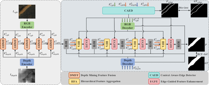
Figure 2: The architecture of the proposed DMENet. DMENet adopts the Swin Transformer in the encoding stage to extract RGB and depth features. A DMFF module generates strengthened RGB-D defect representations via cross-modal interaction. In the decoding stage, the HFA module integrates adjacent RGB-D encoding features with RGB and depth decoding features. Edge-sensitive context from the CAED is embedded into the decoding features via the EGFE module to capture defect details. Abbreviations: DMENet = Depth-Mining Network with Edge-Sensitive Context; DMFF = Depth-Mining Feature Fusion; HFA = Hierarchical Feature Aggregation; CAED = Context-Aware Edge Detector; EGFE = Edge-Guided Feature Enhancement; RFB = Receptive Field Block; BCE = Binary Cross-Entropy; IoU = Intersection over Union; GT = Ground Truth. Please click here to view a larger version of this figure.

Depth-Mining Feature Fusion module
In defect scenes with weak spatial appearances, poor depth data failed to capture spatial differences. Thus, methods based on the undifferentiated bidirectional interaction mode could introduce substantial redundancy that interferes with RGB features^35,36. To address this issue, the DMFF module, as depicted in Figure 3, was proposed to selectively mine valuable information from the depth modality to enrich the defect feature representation, while robustly and sufficiently matching complementary information across modalities.

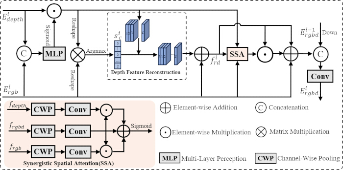
Figure 3: Illustration of the Depth-Mining Feature Fusion module. Abbreviations: DMFF = Depth-Mining Feature Fusion; SSA = Synergistic Spatial Attention; MLP = Multi-Layer Perceptron; CWP = Channel-Wise Pooling; Conv = Convolution. Please click here to view a larger version of this figure.

Firstly, to address inaccuracies in depth features at the pixel level, stable RGB information was used to calibrate depth features, ensuring that spatial depth information was properly adjusted. RGB and depth features were fed into the DMFF module, concatenated along the channel dimension, and then passed through a Multi-Layer Perceptron (MLP) to refine features comprehensively while gradually compressing the channel dimension. After being processed by a sigmoid function, a weight map wⁱ_p was used to calibrate depth features at the pixel level. The process was expressed by the following formula:

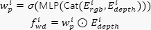 (1)

Where Cat(·) represents the concatenation operation along the channel dimension, and ⊙ represents element-wise multiplication. In this way, a more reliable representation of depth features was provided for subsequent interaction.

Secondly, to robustly exploit the complementary information and reduce the semantic gap between modalities, the DMFF module reconstructed depth features to align them with the semantic information of RGB features at the channel level. The DMFF module dynamically evaluated the semantic value of depth features by correlating them with RGB features and extracting the most semantically relevant features from the depth channels. Concretely, initial RGB and adjusted depth features were reshaped into ℝ^C×N, where N = H×W. A matrix multiplication was performed to generate a channel correlation matrix, quantifying the semantic similarity between depth and RGB features at the channel level. The most correlated depth channel for each RGB channel was identified via an argmax operation, yielding a sequence s_c(i). The corresponding depth channels, in sequence, were extracted and sorted to form reconstructed depth features. These reconstructed depth features were then added to the RGB features, aligning them into a cohesive representation denoted as preliminary RGB-D features fⁱ_rd. The following formula illustrates the process:

 (2)

Where ⊗ represented matrix multiplication. DFR(·) represented the operation of sequentially extracting and combining the most correlated depth channels for each RGB channel to reconstruct depth features.

Thirdly, to emphasize salient regions and reduce spatial inconsistencies across modalities, the SSA module was designed to refine representations by integrating complementary spatial information. The SSA module synergistically leveraged both shared and complementary spatial features from multiple modalities. It not only suppressed irrelevant noise but also improved its focus on mutual critical defect regions. The SSA module first extracted key spatial features using convolution and channel pooling operations. To achieve synergy between modalities, features were combined through element-wise multiplication to emphasize shared information and addition to highlight complementary information. The synergistic spatial attention map w_s was obtained through a sigmoid function. The process was expressed as follows:

 (3)

Where mod ∈ {rgb, depth, rgbd}, and CWP(·) represents the channel-wise pooling operations, while Conv_7×7(·) represents the 7×7 convolution followed by Batch Normalization (BN) and ReLU functions. After that, the preliminary RGB-D features were weighted and added with the input RGB features to obtain fⁱ_wrd. The mathematical expression was: 

 (4)

Finally, these features were concatenated with downsampled features from the previous DMFF module and then convolved. Thus, the RGB-D features Eⁱ_rgbd RGB-only information and depth information were obtained, constructing the RGB-D encoding stream. Generally, the DMFF module achieved precise complementarity of semantic information between the two modalities by mining valuable depth information and exploring commonalities across modalities, thereby generating an RGB-D encoding stream with rich defect representation.

Hierarchical feature aggregation module
Given that surface defects may exhibit subtle features, preserving detailed information was essential for discerning distinctions between defects and their surroundings. The HFA module, as shown in Figure 4, was proposed to aggregate hierarchical features during the decoding stage. The HFA module enriched decoding features through a subdivided sampling process and further utilized modality-specific information to emphasize defect regions.

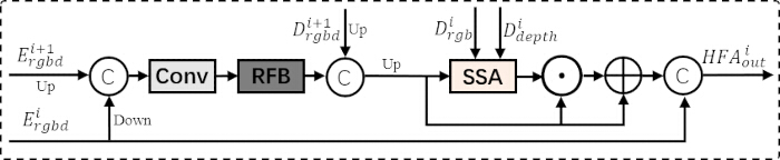
Figure 4: Illustration of the Hierarchical Feature Aggregation module. Abbreviations: HFA = Hierarchical Feature Aggregation; RFB = Receptive Field Block; SSA = Synergistic Spatial Attention; Up = Up-sampling; Down = Down-sampling; Conv = Convolution. Please click here to view a larger version of this figure.

To effectively capture defect details, the decoding features were enriched with contextual information and progressively refined to ensure smooth feature restoration. Adjacent encoding features were sampled to an intermediate resolution and fused through convolution, creating a unified multi-level representation. The features were processed by the RFB module to capture multi-scale information and reduce channel redundancy. Then, they were concatenated with up-sampled high-level decoding features to enrich them. Further up-sampling progressively restored the resolution of the feature map, obtaining . This procedure was captured by the following formula:

 (5)

Furthermore, inspired by SPNet²⁴, the modality-specific information within the triple-stream architecture was leveraged to emphasize defect regions. To mitigate differences in feature distributions and reduce interference from redundant information in specific modalities, the SSA module was employed to indirectly focus on mutually salient regions across modalities. It emphasized defect regions while reducing irrelevant information that could arise during progressive sampling. Finally, they were concatenated with the skip connection features from the encoder to generate HFAⁱ_out. Thus, the HFA module aggregated hierarchical features to preserve detailed defect information while focusing on salient defect regions across modalities, ensuring that fine details and modality-specific information were fused to capture a subtle defect representation.

Edge-prior module
Context-aware edge detector
Superior edge information provided a guarantee for boundary refinement, which was critical for precise defect localization. The CAED in Figure 5 leveraged multi-level features to comprehensively model edge information³⁷. It further exploited the unique characteristics of each modality in defect scenes: shallow RGB features effectively captured surface textures and color variations, while depth features typically localized defect regions only vaguely at deeper semantic levels. By exploring complementarity across modalities, the CAED delivered reliable edge information for boundary refinement.

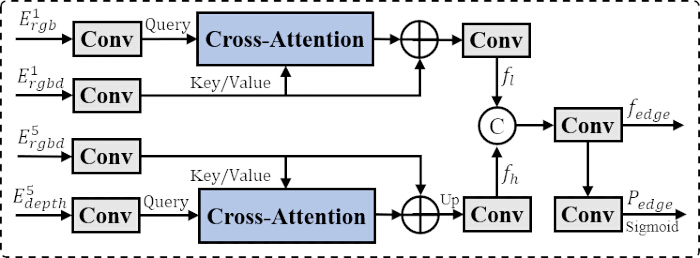
Figure 5: Illustration of the Context-Aware Edge Detector. Abbreviations: CAED = Context-Aware Edge Detector; Conv = Convolution; Up = Up-sampling. Please click here to view a larger version of this figure.

Specifically, the cross-attention mechanism was employed to model long-range dependencies across different modalities³⁸, enabling the module to focus on their complementary information within a global context. Convolutions were applied to compress the low-level RGB and RGB-D features. The cross-attention layer then refined these features by emphasizing salient texture details shared between the modalities, followed by another convolution to extract low-level features f_l ∈ ℝ^64×H×W. For high-level features, the same cross-attention mechanism was used to complement semantic information between RGB-D and depth features, resulting in high-level features f_h ∈ ℝ^256×H×W. The process was expressed in the following formula:

 (6)

Where the RGB or depth features were used as the query and the RGB-D features as the key and value.

Next, low-level and high-level features were combined to model object-related edge information, leveraging both texture details and general semantic information to capture defect boundaries. The low-level features and up-sampled high-level features were concatenated, and convolutions were applied to produce f_edge ∈ ℝ^256×H×W, which was rich in contextual information and highly sensitive to edges, and closely supervised with edge ground truth. After further convolution processing and the operation of a sigmoid function, the edge maps P_edge ∈ ℝ^1×H×W were obtained, which explicitly highlighted the defect boundary regions. The following formula describes the above operations:

 (7)

The CAED combined low-level textural details and high-level semantic information across specific modalities. It generated fine-grained edge maps and coarse-grained, context-sensitive edge features, supporting the comprehensive refinement of defect boundaries.

Edge-guided feature enhancement module
Though fine-grained spatial weighting was a common edge-prior method, it struggled to fundamentally capture the semantic distinctions between defect boundaries and their surroundings. Accordingly, as illustrated in Figure 6, the EGFE module was designed. This module not only sharpened defect boundaries using fine-grained edge maps but also integrated coarse-level, edge-sensitive contextual features to detect boundary formation.

Figure 6: Illustration of the Edge-Guided Feature Enhancement module. Abbreviations: EGFE = Edge-Guided Feature Enhancement; HFA = Hierarchical Feature Aggregation; MLP = Multi-Layer Perceptron; GAP = Global Average Pooling; Conv1d = 1-Dimensional Convolution. Please click here to view a larger version of this figure.

Contextual edge-sensitive features were integrated into the decoding process to enhance the perception of defect boundaries by grasping both global and local information. Specifically, edge features were matched with local RGB-D decoding features via an MLP to ensure compatibility, and then fused element-wise to detect defect boundaries at coarse granularity. A residual connection was then introduced to preserve local information, obtaining fⁱ_e. This procedure was articulated through the following equation:

 (8)

Thus, the EGFE module perceived the division between defects and backgrounds at a broader feature level.

Intuitive edge maps were introduced to sharpen defect boundaries at a fine granularity. The edge maps were sampled to match the resolution of fⁱ_e and multiplied with them, enhancing the edge-related regions within the features. Then, a residual connection was added, followed by a convolution to generate f̃ⁱ_e. This process was formulated as:

 (9)

To enhance the feature representation of the defect boundaries, a local channel attention mechanism that selectively emphasized the significant channels was applied to f̃ⁱ_e by performing localized cross-channel interactions, similar to the research³⁷. It captured the overall significance of each channel by weighting them based on their contribution to the defect boundary. The resulting features were weighted as the output of the EGFE module. Mathematically, it was expressed as:

 (10)

Where Conv1D_k represents the 1D convolution with a kernel size of k, following the settings in the research³⁹. In this way, the EGFE module refined the decoding features by integrating edge-sensitive context and edge maps. The coarse-grained context offered a broader understanding of the scene's semantics to define boundaries, while the fine-grained edge maps provided detailed delineation of defect contours, leading to comprehensive and precise refinement of defect boundaries.

Loss function
As in most prior work, the hybrid loss was used, combining Binary Cross-Entropy (BCE) and Intersection over Union (IoU) losses. The defect prediction consisted of three parts: P_rgb, P_depth, which were produced by the final decoding layers of the RGB and depth modalities, and Pⁱ_rgbd (i=1,2,3,4,5), which were generated by multiple RGB-D decoding layers. Employing a deep supervision strategy in the RGB-D modality minimized information loss and facilitated gradient propagation. These losses were expressed by the following formula:

 (11)

Where l_bce denotes the BCE loss, l_iou denotes the IoU loss, and G denotes the ground truth.

Additionally, the Dice loss was employed to supervise the predicted edge maps P_edge, which offered superior noise resistance and adaptability to class imbalance. It was expressed as follows:

 (12)

Where l_dice denotes the Dice loss, and G_edge denotes the edge ground truth.

In summary, the total loss was represented as follows:

 (13)

Dataset preparation
The NEU RSDDS-AUG dataset was used to evaluate the proposed method for surface defect detection³⁰. It comprised 1,862 RGB-D image pairs captured from the P60 rail, with depth data acquired using a binocular stereo vision system. The dataset featured image pairs depicting scratches and holes of various scales, categorized as single-defect or multiple-defect. Furthermore, DMENet was tested on three RGB-D benchmark datasets, NLPR⁴⁰, NJU2K⁴¹, and STERE⁴², to demonstrate its generalization capability in diverse natural scenes. NLPR consisted of 1000 RGB-D image pairs captured using a Microsoft Kinect camera in various settings and calibrated for depth. NJU2K contained 1,985 image pairs from the Internet and 3D movies, with depth maps generated via optical flow. STERE comprised 1,000 image pairs downloaded from the Internet with depth images estimated by optical flow. The training set included 2,185 image pairs from NJU2K and NLPR, with 220 image pairs for validation; the remaining pairs were used for testing.

Implementation details
DMENet was developed using the deep learning framework PyTorch. The model was trained and tested using the same hardware configuration. Swin-S was used as the backbone, with parameters initialized using the ImageNet-22k pretrained weights. AdamW was selected as the optimizer, with the weight decay set to 0.01. The initial learning rate was set to 1e-4 and decreased by a factor of 0.1 every 70 epochs. The training phase used a batch size of 8 and ran for 150 epochs. The input image resolution was 224 × 224.

Data augmentation was applied randomly to each training image, including random horizontal flipping with a probability of 0.5, random rotation in the range -15° to 15° with a probability of 0.2, and random cropping with a border of 20 and a ratio in the range (0.6, 1.0). The random seed was set to 42 for reproducibility. All input images were normalized using ImageNet mean and standard deviation.

For the NEU RSDDS-AUG dataset, the training set contained 1,500 images, and the validation set contained 362 images (a random 80/20 split with a fixed seed of 42). The best model checkpoint was selected based on the lowest validation MAE (evaluated every 5 epochs). The test set (362 images) was used only for final evaluation and was never used during model selection.

Model training
Five widely recognized key metrics were used to measure the performance of DMENet. These metrics included Mean Absolute Error (MAE)⁴³, S-Measure (S_α)⁴⁴, E-Measure (E_φ)⁴⁵, F-Measure (F_β)⁴⁶, and Precision-Recall (P-R) curve⁴⁷.

Mean Absolute Error (MAE): MAE measures the average absolute difference between the prediction map and the ground truth, quantifying the discrepancy between them. A lower MAE indicates that the predicted saliency map is closer to the ground truth:

 (14)

Where N is the total number of pixels, p_i is the value of the i-th pixel in the predicted saliency map, and g_i is the value of the i-th pixel in the true saliency map.

S-Measure (S_α): S-Measure evaluates the structural similarity between the prediction map and the ground truth by focusing on region similarity and object similarity. Region similarity assesses the consistency of saliency across various image regions, while object similarity examines the prominence with which main objects are depicted:

 (15)

S_o denotes object similarity, S_r represents region similarity, and α is a parameter that balances the two, typically set at 0.5.

F-Measure (F_β): The F-Measure provides a comprehensive and intuitive evaluation of the model’s overall performance by synthesizing precision and recall metrics:

 (16)

Where β² is predetermined and typically set at 0.3. The max F-Measure F^max_β was used to assess the model's performance under the optimal threshold setting.

E-Measure (E_φ): E-Measure incorporates both local and global information to evaluate the model, focusing on differences in local pixel data relative to the global averages:

 (17)

φ(u,v) is the enhanced alignment matrix, indicating the correlation between the prediction map and the ground truth after adjustment for their global mean values. The max E-Measure (E^max_φ) was employed to quantitatively assess the model's performance under the optimal threshold setting.

Precision-Recall (P-R): By binarizing the prediction map P at various thresholds to produce binary maps B and comparing these with the corresponding ground truth G, a set of precision and recall scores was computed:

 (18)

Risultati

Mechanism differentiation from RGB-D methods
Architectural comparison
To clarify the methodological positioning of DMENet, the comparison with three representative RGB-D methods (SPNet, PICRNet, and SAINet) is summarized below. The comparison covers backbone selection, cross-modal fusion mechanism, spatial attention strategy, hierarchical aggregation, and edge handling. The proposed DMENet introduces several distinct design choices that differentiate it from existing approaches.

Specifically, the Depth-Mining Feature Fusion (DMFF) module implements selective mining through pixel-level calibration and channel-level alignment (Eqs. 1-2), in contrast to the simple feature concatenation used in SPNet and PICRNet. The Synergistic Spatial Attention (SSA) module detects regions where RGB and depth modalities agree on defect locations, rather than relying on per-modality attention as in PICRNet. The Edge-prior Module (combining CAED and EGFE) provides dual-granularity edge refinement, a feature absent in all compared methods. The full architectural comparison is provided in Supplementary File 1.

The methodological positioning of DMENet is further clarified by its target domain. SPNet and PICRNet were originally designed for RGB-D salient object detection in natural scenes, while SAINet focuses on rail surface defects. DMENet is specifically designed for industrial surface defect segmentation, providing a coherent framework that integrates selective depth mining, hierarchical feature aggregation, and edge-sensitive context. Figure 7 presents a side-by-side architectural comparison of DMENet with SPNet and PICRNet, highlighting the differences in fusion strategy, spatial attention, and edge handling.

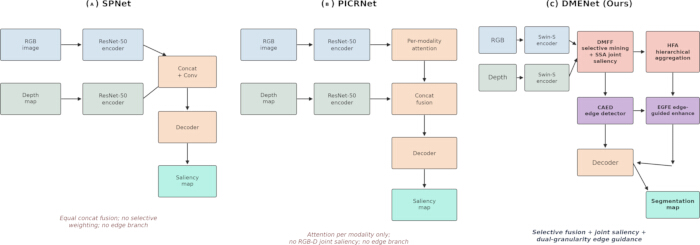
Figure 7: Architectural comparison of DMENet with representative RGB-D methods. (A) SPNet. (B) PICRNet. (C) DMENet (the proposed method). DMENet differs in three aspects: selective depth-mining fusion with joint RGB-D saliency rather than simple concatenation, hierarchical aggregation, and dual-granularity edge guidance (CAED + EGFE), which is absent from both baselines. Abbreviations: SPNet = Specificity-Preserving Network; PICRNet = Point-Aware Interaction and CNN-Induced Refinement Network; DMENet = Depth-Mining Network with Edge-Sensitive Context; DMFF = Depth-Mining Feature Fusion; SSA = Synergistic Spatial Attention; HFA = Hierarchical Feature Aggregation; CAED = Context-Aware Edge Detector; EGFE = Edge-Guided Feature Enhancement. Please click here to view a larger version of this figure.

Comparison with state-of-the-art methods
To validate the effectiveness of DMENet, comparison experiments are conducted on 18 state-of-the-art RGB-D-based methods. These include BTSNet⁴⁸, TriTranNet⁴⁹, SPNet²⁴, C²DFNet⁵⁰, CIRNet²⁵, RFNet⁵¹, CLANet³⁰, FHENet¹¹, MENet¹⁴, PENet³⁵, PICRNet¹⁶, CAVER⁵², RDNet³⁶, SAINet³², HFMDNet¹⁷, SA2F⁴³, ACLNet-T¹², and TCINet¹³. For methods^{16,24,25,48,49,50,51,52} not using the NEU RSDDS-AUG dataset, parameter settings as described in their original papers, and the same data division strategy are implemented. For methods^11,32,36, which use this publicly available dataset, they are reevaluated using the prediction maps provided by the authors. For methods^{14,17,30,35,53} that use the dataset and are not publicly available, experimental results published in the corresponding papers are referred.

Quantitative evaluation
As shown in Table 1, DMENet outperforms state-of-the-art comparison methods in four evaluation metrics, achieving the best performance. Compared to HFMDNet¹⁷, DMENet exceeds it by 7.8%, 0.6%, and 0.2% in MAE, S_α, and E^max_φ, respectively. When compared to CLANet³⁰, a pioneering method specifically designed for the NEU RSDDS-AUG dataset, the improvements are noticeable: 31.9% in MAE, 4.0% in S_α, 2.8% in E^max_φ, and 3.9% in F^max_β. Among the methods specifically designed for the NEU RSDDS-AUG defect dataset, RDNet³⁶ performs the best. DMENet outperforms RDNet by 16.1% in MAE, 0.7% in S_α, 0.9% in E^max_φ, and 0.9% in F^max_β, making a significant advancement over previous methods.

Method	Publication	MAE lower is better	S-measure higher is better	Max E-measure higher is better	Max F-measure higher is better
BTSNet	ICME 2021	0.066	0.845	0.917	0.898
TriTransNet	ACM MM 2021	0.07	0.833	0.915	0.889
SPNet	ICCV 2021	0.065	0.84	0.921	0.897
C2DFNet	TMM 2022	0.096	0.801	0.877	0.86
CIRNet	TIP 2022	0.086	0.828	0.894	0.856
RFNet	3DV 2022	0.063	0.842	0.923	0.899
CLANet	TMECH 2022	0.069	0.834	0.921	0.877
FHENet	TIM 2023	0.063	0.838	0.926	0.882
MENet	TCSVT 2023	0.057	0.856	0.939	0.899
PENet	TIM 2023	0.054	0.859	0.94	0.905
PICRNet	ACM MM 2023	0.053	0.857	0.936	0.908
CAVER	TIP 2023	0.055	0.859	0.935	0.91
RDNet	TASAE 2024	0.056	0.861	0.939	0.903
SAINet	OPTLASERENG 2024	0.055	0.851	0.936	0.898
HFMDNet	TIM 2024	0.051	0.862	0.945	0.911
SA2F	TII 2024	0.061	0.845	0.927	0.883
ACLNet-T	TNNLS 2025	0.056	0.86	0.938	0.898
TCINet	TIM 2025	0.049	0.861	0.937	0.901
Ours	-	0.047	0.867	0.947	0.911

Table 1: Quantitative comparisons on the NEU RSDDS-AUG dataset. Performance evaluation across four metrics compared against 18 state-of-the-art methods. ” ↑ ”/” ↓” indicates that larger or smaller is better. The best result for each metric is highlighted in bold. Abbreviations: NEU RSDDS-AUG = Northeastern University Rail Surface Defect Detection System Augmented Dataset; MAE = Mean Absolute Error (lower is better); S_α = Structural Measure (higher is better); E^max_φ = Maximum Enhanced-Alignment Measure (higher is better); F^max_β = Maximum F-Measure (higher is better); SOTA = State-of-the-Art.

Figure 8 illustrates the Precision-Recall (P-R) and F-Measure curves for DMENet compared with other methods. The P-R curves depict how precision varies with recall across different methods. The P-R curve of DMENet is stable and balanced, positioned closest to the top-right of the graph, indicating that it maintains the highest precision under the same recall rate. The F-Measure curves show F-Measure across various thresholds. The DMENet curve consistently remains above those of the other methods, indicating it maintains the best F-Measure performance across different thresholds.

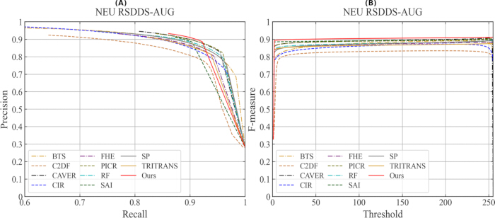
Figure 8: The P-R curves and F-Measure curves on the NEU RSDDS-AUG dataset. (A) P-R curves of DMENet compared to other methods. (B) F-measure curves at various thresholds. Abbreviations: P-R = Precision-Recall; NEU RSDDS-AUG = Northeastern University Rail Surface Defect Detection System Augmented Dataset. Please click here to view a larger version of this figure.

Visualization analysis
Figure 9 compares ground truth (GT) and the visual results of the proposed method with those of other methods. In rows 1, 2, 5, 8, and 9, when the textures and color appearances of the background and defects are highly similar, other methods are more prone to misidentifying the background as defects. In contrast, DMENet effectively uses depth information to distinguish foreground from background, thereby reducing misidentification. Furthermore, as shown in rows 3, 4, 7, and 8, the proposed method effectively bridges the semantic gap across modalities, reduces semantic confusion, and demonstrates enhanced robustness to disruptions caused by poor depth information. Compared with the comparative methods, the predictions of DMENet exhibit more complete internal structures, smoother boundaries, and better separation, which closely resemble the true morphology of irregular defects, as seen in rows 3, 4, 5, and 6. These results highlight the effectiveness of the proposed method in handling challenging defect scenes compared to other methods.

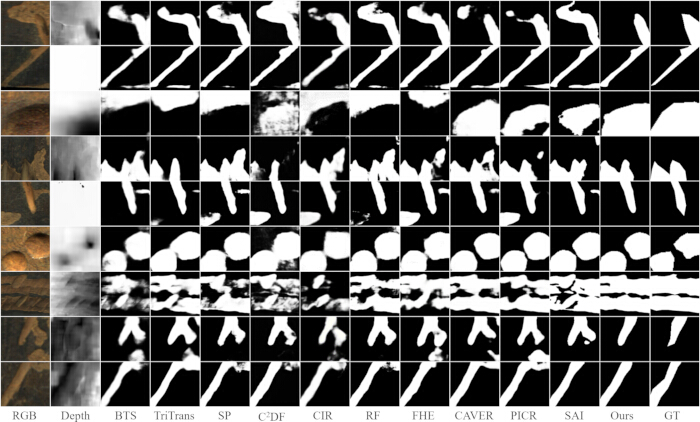
Figure 9: Visual comparisons for prediction maps of different methods on the NEU RSDDS-AUG dataset. Abbreviations: RGB = Red-Green-Blue; Depth = Depth Map; BTS = BTSNet; TriTrans = TriTransNet; SP = SPNet; C2DF = C2DFNet; CIR = CIRNet; RF = RFNet; FHE = FHENet; CAVER = Cross-Modal View-Mixed Transformer; PICR = PICRNet; SAI = SAINet; Ours = DMENet; GT = Ground Truth. Please click here to view a larger version of this figure.

Complexity evaluation
To assess the computational efficiency of the proposed method, a thorough evaluation of its complexity compared to various methods on the same device is conducted. This assessment encompasses several critical metrics, including parameters, floating-point operations (FLOPs), and inference speed (FPS). As illustrated in Table 2, DMENet delivers performance that surpasses more complex models while maintaining moderate FLOPs, parameters, and FPS. Therefore, the proposed method achieves a relatively good balance between resource usage and performance, making it a viable option for the application in defect scenes that require both efficiency and effectiveness.

Model	Input Size	FLOPs G lower is better	Params M lower is better	FPS higher is better
BTSNet	352 x 352	250.8	99	17.2
TriTransNet	256 x 256	282.7	138.8	8.9
SPNet	352 x 352	68.1	150.3	41
C2DFNet	256 x 256	11.1	47.5	193.2
CIRNet	352 x 352	42.6	103.2	66.4
RFNet	352 x 352	37.3	90.8	31.2
FHENet	320 x 320	2.8	5.2	170.7
MENet	384 x 384	50.7	183.6	-
PENet	320 x 320	32.2	82.4	-
PICRNet	224 x 224	27.1	112	57.9
CAVER	256 x 256	31.6	93.8	83.7
RDNet	320 x 320	40.3	87.7	-
SAINet	256 x 256	33.1	57.9	81.6
HFMDNet	384 x 384	242.2	431.6	-
Ours	224 x 224	28.4	134.1	56.2

Table 2: Comparisons of computational efficiency and complexity on the NEU RSDDS-AUG dataset. Evaluation of model resource usage measured on a standardized hardware environment. Abbreviations: NEU RSDDS-AUG = Northeastern University Rail Surface Defect Detection System Augmented Dataset; FLOPs = Floating-Point Operations; G = Giga (10⁹); Params = Parameters; M = Millions (10⁶); FPS = Frames Per Second (higher is better).

Ablation studies
Ablation studies are conducted on the NEU RSDDS-AUG dataset to validate the effectiveness of each component in DMENet.

Effectiveness of each component in DMENet
In the baseline, the CAED, EGFE, and HFA modules are removed from the original DMENet framework, and the DMFF module is replaced with element-wise addition to enable simple cross-modal interaction. The following variants are set to evaluate the contribution of the proposed modules: (1) Baseline with DMFF module for cross-modal interaction; (2) Baseline with DMFF module and HFA for feature aggregation; (3) Complete network that includes DMFF, HFA, CAED, and EGFE modules for boundary refinement. It should be noted that CAED and EGFE function as interconnected modules, and they are either included or removed together in the ablation studies. The quantitative results and visual results are shown in Table 3 and Figure 10, respectively.

Setting	Baseline	DMFF	HFA	CAED and EGFE	MAE lower is better	S-measure higher is better	Max E-measure higher is better	Max F-measure higher is better
S1	Yes	No	No	No	0.056	0.847	0.936	0.895
S2	Yes	Yes	No	No	0.051	0.858	0.943	0.903
S3	Yes	Yes	Yes	No	0.05	0.859	0.945	0.905
Ours	Yes	Yes	Yes	Yes	0.047	0.867	0.947	0.911

Table 3: Module ablation analysis on the NEU RSDDS-AUG dataset. Quantitative performance contributions of progressively incorporating DMFF, HFA, and CAED with EGFE modules into the baseline model. Abbreviations: NEU RSDDS-AUG = Northeastern University Rail Surface Defect Detection System Augmented Dataset; Baseline = Simple addition fusion model; DMFF = Depth-Mining Feature Fusion; HFA = Hierarchical Feature Aggregation; CAED = Context-Aware Edge Detector; EGFE = Edge-Guided Feature Enhancement; MAE = Mean Absolute Error (lower is better); S_α = Structural Measure (higher is better); E^max_φ = Maximum Enhanced-Alignment Measure (higher is better); F^max_β = Maximum F-Measure (higher is better).

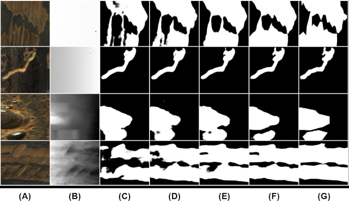
Figure 10: Visual comparisons for prediction maps generated by different settings on modules. (A) RGB. (B) Depth. (C) S1. (D) S2. (E) S3. (F) Ours. (G) GT. Abbreviations: RGB = Red-Green-Blue; Depth = Depth Map; S1 = Baseline without DMFF, HFA, CAED, EGFE; S2 = Baseline with DMFF; S3 = Baseline with DMFF and HFA; Ours = Full DMENet Model; GT = Ground Truth. Please click here to view a larger version of this figure.

DMENet achieves improvements of 16.1% in MAE, 2.4% in S_α, 1.2% in E^max_φ and 1.8% in F^max_β compared to the baseline in total, demonstrating overall advancements in detection performance. Compared to the simple interaction method, the DMFF module achieves a superior cross-modal interaction effect. It can be seen that DMENet reduces semantic inconsistencies and resists interference from redundant depth information, which effectively improves the identification of defect regions. The HFA module aggregates hierarchical features to preserve defect details and to complement salient regions across modalities, resulting in complete, clear defect predictions. With the CAED and EGFE modules, the boundary refinement process comprehensively incorporates edge information at both coarse and fine levels, making defect boundaries more distinct and achieving the finer separation between foreground and background regions.

Effectiveness of each module's internal structure
As shown in Table 4, to further analyze how each design contributes, ablation experiments are conducted on the internal design structures of each module. Experiments are performed with the following settings: (1) Without pixel-level calibration of depth features in the DMFF module. (2) Replacing depth reconstruction with element-wise addition for cross-modal interaction in the DMFF module. (3) Without skip connections from adjacent encoding layers for feature aggregation in the HFA module. (4) Replacing CAED with a concatenation of shallow features followed by convolutions. (5) Without edge-sensitive context for boundary perception in the EGFE module. (6) Without edge maps for boundary sharpening in the EGFE module. Table 4 shows the quantitative results, and Figure 11 illustrates the visual results.

Module	Setting	MAE lower is better	S-measure higher is better	Max E-measure higher is better	Max F-measure higher is better
DMFF	without pixel calibration	0.049	0.866	0.944	0.907
DMFF	without channel alignment	0.051	0.862	0.942	0.904
HFA	without encoding connections	0.048	0.866	0.947	0.909
CAED and EGFE	without CAED	0.049	0.863	0.944	0.905
CAED and EGFE	without context features	0.049	0.865	0.945	0.908
CAED and EGFE	without edge maps	0.048	0.867	0.947	0.91
Ours	Ours	0.047	0.867	0.947	0.911

Table 4: Module internal structure ablation analysis on the NEU RSDDS-AUG dataset. Evaluation of specific structural design choices within the DMFF, HFA, CAED, and EGFE modules. Abbreviations: NEU RSDDS-AUG = Northeastern University Rail Surface Defect Detection System Augmented Dataset; w/o = Without; DMFF = Depth-Mining Feature Fusion; HFA = Hierarchical Feature Aggregation; CAED = Context-Aware Edge Detector; EGFE = Edge-Guided Feature Enhancement; MAE = Mean Absolute Error (lower is better); S_α = Structural Measure (higher is better); E^max_φ = Maximum Enhanced-Alignment Measure (higher is better); F^max_β = Maximum F-Measure (higher is better).

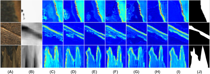
Figure 11: Visualization comparison for feature maps of the last decoding stage by different settings on model internal structures. (A) RGB. (B) Depth. (C) w/o pixel calibration. (D) w/o channel alignment. (E) w/o encoding connections. (F) w/o CAED. (G) w/o context features. (H) w/o edge maps. (I) Ours. (J) GT. Abbreviations: w/o = Without; RGB = Red-Green-Blue; Depth = Depth Map; CAED = Context-Aware Edge Detector; Ours = Full DMENet Model; GT = Ground Truth. Please click here to view a larger version of this figure.

When the DMFF module introduces depth features without pixel-wise calibration, additional noise from the depth information appears. Depth pixel-wise calibration provides a reliable spatial representation of depth features for subsequent fusion. When the depth feature reconstruction operation in the DMFF module is removed, irrelevant channel information in the depth features leads to incorrect predictions. This operation is used to mine valuable depth information that is semantically related to RGB and aligns the semantics between the modalities at the channel level. When skip connections in the HFA module are removed, defect features become incomplete and distorted. They are introduced to fuse multi-scale features with contextual information, thereby enhancing the richness of the feature representation and retaining more defect details.

When the CAED is replaced with a typical method that concatenates RGB and depth features from the shallow layers using convolutions, the resulting features contain more noise, and the predicted defect edges deviate from the ground truth. The CAED can provide higher-quality edge information, ensuring the effectiveness of the boundary refinement process. To validate this claim, Figure 12 shows the edge maps obtained using different methods. It can be seen that the CAED can produce higher-quality edge maps. Furthermore, in the EGFE module, removing edge-sensitive context features while retaining edge maps results in incorrectly localized defect boundaries, and the separation between foreground and background becomes less distinct. Conversely, eliminating edge map features leads to a relatively light impact. In this case, some defect edge regions in the features become slightly blurred, but the separation between foreground and background is still clear. Compared with directly sharpening defect boundaries using edge maps, edge-sensitive contextual features can separate the foreground and background at a broader semantic level, better perceive defect boundary regions, and have a more significant impact on the results.

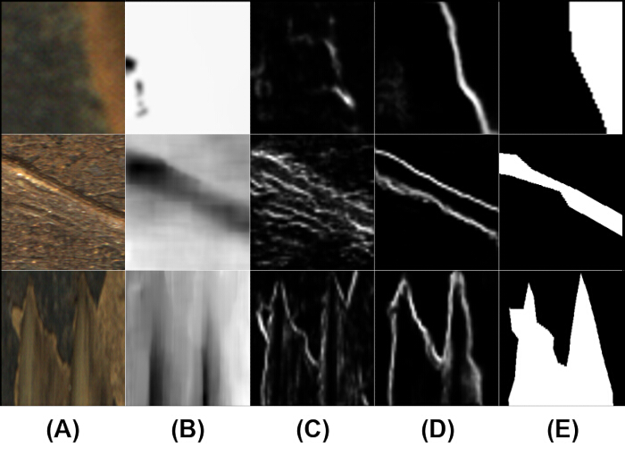
Figure 12: Visualization comparison for edge maps by different settings on edge detector. (A) RGB. (B) Depth. (C) w/o CAED. (D) Ours. (E) GT. Abbreviations: w/o = Without; CAED = Context-Aware Edge Detector; RGB = Red-Green-Blue; Depth = Depth Map; Ours = Full DMENet Model; GT = Ground Truth. Please click here to view a larger version of this figure.

Effectiveness of each modality
Ablation studies are also conducted on different modalities to determine whether the proposed method effectively utilizes complementary information between modalities. Experiments are conducted using either RGB or depth as input while preserving all components of DMENet. As shown in Table 5 and Figure 12, DMENet outperforms the single RGB modality setup by 9.6% in MAE, 0.6% in S_α, 0.7% in E^max_φ, and 0.9% in F^max_β. When the color and texture of the defect surface are highly similar, a single RGB modality cannot clearly distinguish the foreground from the background. Furthermore, DMENet significantly surpasses the single depth modality setup by 62.7% in MAE, 20.6% in S_α, 14.0% in E^max_φ, and 19.2% in F^max_β. It can be seen that depth information is poor, and defect-related information is severely limited, which is a common issue in defect scenes. These results indicate that across the entire NEU RSDDS-AUG dataset, the RGB modality provides richer, more accurate defect information and plays a dominant role in surface defect detection. While primarily leveraging RGB information, RGB-D modality in DMENet introduces supplementary depth information to enhance RGB features. DMENet not only improves detection accuracy based on good-depth cases but also maintains robustness in poor-depth cases.

Setting	MAE lower is better	S-measure higher is better	Max E-measure higher is better	Max F-measure higher is better
Depth	0.126	0.719	0.831	0.764
RGB	0.052	0.862	0.94	0.903
RGB-D	0.047	0.867	0.947	0.911

Table 5: Modality ablation analysis on the NEU RSDDS-AUG dataset. Comparison of network performance using single depth, single RGB, and combined RGB-D modalities. Abbreviations: NEU RSDDS-AUG = Northeastern University Rail Surface Defect Detection System Augmented Dataset; RGB = Red-Green-Blue; D = Depth; MAE = Mean Absolute Error (lower is better); S_α = Structural Measure (higher is better); E^max_φ = Maximum Enhanced-Alignment Measure (higher is better); F^max_β = Maximum F-Measure (higher is better).

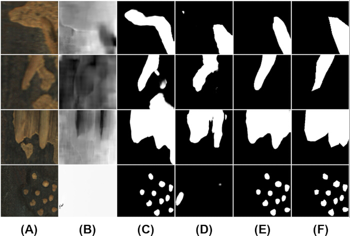
Figure 13: Visual comparisons for prediction maps generated by different settings on modalities. (A) RGB. (B) Depth. (C) RGB-based prediction. (D) Depth-based prediction. (E) RGB-D-based prediction. (F) GT. Abbreviations: RGB = Red-Green-Blue; Depth = Depth Map; RGB-D = Combined RGB and Depth Modalities; GT = Ground Truth. Please click here to view a larger version of this figure.

Effectiveness of loss weighting
As shown in Table 6, to provide empirical support for the loss weighting design, ablation experiments were conducted with four combinations of the three loss components (L_bce : L_iou : L_dice): the baseline setting (1:1:1), weak edge supervision (1:1:0.5), strong edge supervision (1:1:2.0), and high BCE weight (2:1:1). All variants were trained on NEU RSDDS-AUG under identical settings (warm start, 10 epochs).

Variant	Lbce : Liou : Ldice	MAE lower is better
baseline_w11	1 : 1 : 1	0.0491
weak_dice	1 : 1 : 0.5	0.0496
strong_dice	1 : 1 : 2.0	0.0489
high_bce	2 : 1 : 1	0.0501

Table 6: Loss weight ablation on NEU RSDDS-AUG under warm-start training. Performance sensitivity across four loss weighting ratios (L_bce : L_iou : L_dice) evaluated on 10 epochs. Abbreviations: NEU RSDDS-AUG = Northeastern University Rail Surface Defect Detection System Augmented Dataset; BCE = Binary Cross-Entropy Loss; IoU = Intersection over Union Loss; Dice = Dice Loss; MAE = Mean Absolute Error (lower is better).

The four variants achieve MAE of 0.0491, 0.0496, 0.0489, and 0.0501, respectively. The differences are within 0.0012, indicating that DMENet is not sensitive to the exact loss weighting. The strong edge supervision setting (1:1:2.0) achieves the best result, suggesting that edge supervision (Dice loss on edge maps) contributes marginally more than the other components, consistent with the design philosophy of edge-guided refinement. The baseline 1:1:1 setting is retained in the main experiments for simplicity and to avoid overfitting the hyperparameters to the validation set.

Performance on other datasets
As the NEU RSDDS-AUG dataset lacks a validation set, the generalization capability of DMENet requires further proof. To demonstrate that the proposed method generalizes, experiments are conducted on three additional RGB-D benchmark datasets: NLPR, NJU2K, and STERE. To ensure fairness and enable sufficient comparison, an effort is made to reference the same experimental settings as those used for methods in natural scenes, leading to the removal of some methods evaluated on the NEU RSDDS-AUG dataset and the inclusion of additional methods. The proposed method is compared with 12 state-of-the-art methods, including HAINet⁵⁴, BBSNet⁵⁵, TriTransNet⁴⁹, SPNet²⁴, SiaTrans⁵⁶, C²DFNet⁵⁰, RFNet⁵¹, MITFNet⁵⁷, HiDANet²⁶, CAVER⁵², RDNet³⁶, and TSVT⁵⁸.

As shown in Table 7, DMENet achieves the best result on the NLPR and NJU2K datasets. Specifically, on the NLPR dataset, DMENet surpasses MITFNet⁵⁷, which is the second-best performer, by 5.6% in MAE, 0.5% in S_α, 0.5% in E^max_φ, and 0.3% in F^max_β. On the NJU2K dataset, the proposed approach shows improvements over HiDANet²⁶ by 10.3% in MAE, 0.2% in S_α, and 0.4% in E^max_φ. On the STERE dataset, the overall performance of DMENet surpasses most compared methods, having the best results in MAE and E^max_φ. NLPR, NJU2K, and STERE datasets encompass a variety of natural scenes and diverse salient targets. DMENet demonstrates excellent performance on these datasets, which are characterized by their wide range of salient targets and scenes. As shown in Figure 13, DMENet outperforms other methods across various scenes. The method achieves this by mining valuable depth information and suppressing redundant interference. It also aligns features in different modalities at both the spatial and channel levels to enhance semantic consistency. Thus, it can robustly and effectively synthesize complementary information from modalities across various scenes, achieving superior visual results, as shown in Figure 14.

Method	NLPR MAE lower is better	NLPR S-measure higher is better	NLPR Max E-measure higher is better	NLPR Max F-measure higher is better	NJU2K MAE lower is better	NJU2K S-measure higher is better	NJU2K Max E-measure higher is better	NJU2K Max F-measure higher is better	STERE MAE lower is better	STERE S-measure higher is better	STERE Max E-measure higher is better	STERE Max F-measure higher is better
HAINet	0.024	0.924	0.96	0.915	0.038	0.912	0.944	0.915	0.04	0.907	0.944	0.906
BBSNet	0.023	0.93	0.961	0.918	0.035	0.921	0.949	0.92	0.041	0.908	0.942	0.903
TriTransNet	0.02	0.928	0.966	0.924	0.03	0.92	0.955	0.926	0.033	0.908	0.953	0.911
SPNet	0.021	0.927	0.962	0.919	0.028	0.924	0.952	0.928	0.037	0.907	0.942	0.906
SiaTrans	0.024	0.929	0.964	0.918	0.035	0.923	0.956	0.921	0.038	0.911	0.951	0.907
C2DFNet	0.022	0.928	0.961	0.917	0.039	0.908	0.943	0.909	0.038	0.902	0.943	0.897
RFNet	0.02	0.931	0.966	0.927	0.03	0.925	0.955	0.929	0.036	0.911	0.95	0.911
MITFNet	0.018	0.933	0.968	0.928	0.03	0.923	0.957	0.926	0.034	0.909	0.953	0.91
HiDANet	0.021	0.929	0.963	0.923	0.029	0.926	0.957	0.931	0.035	0.911	0.949	0.912
CAVER	0.021	0.934	0.97	0.929	0.029	0.925	0.959	0.928	0.032	0.917	0.955	0.916
RDNet	0.019	0.936	0.97	0.927	0.034	0.921	0.951	0.924	0.033	0.921	0.955	0.916
TSVT	0.021	0.935	0.966	0.924	0.037	0.917	0.939	0.917	0.035	0.912	0.946	0.915
Ours	0.017	0.938	0.973	0.931	0.026	0.928	0.961	0.931	0.032	0.915	0.956	0.913

Table 7: Quantitative comparisons on benchmark datasets (NLPR, NJU2K, and STERE). Cross-domain performance evaluation against 12 state-of-the-art methods. The best result for each dataset is highlighted in bold. Abbreviations: NLPR = National Laboratory of Pattern Recognition Dataset; NJU2K = Nanjing University 2000 Dataset; STERE = Stereoscopic Dataset; MAE = Mean Absolute Error (lower is better); S_α = Structural Measure (higher is better); E^max_φ = Maximum Enhanced-Alignment Measure (higher is better); F^max_β = Maximum F-Measure (higher is better).

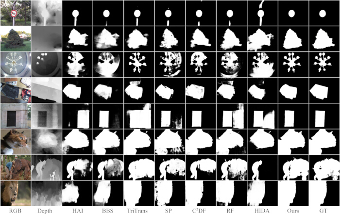
Figure 14: Visual comparisons for prediction maps of different methods on other datasets. Abbreviations: RGB = Red-Green-Blue; Depth = Depth Map; HAI = HAINet; BBS = BBSNet; TriTrans = TriTransNet; SP = SPNet; C2DF = C2DFNet; RF = RFNet; HIDA = HiDANet; Ours = DMENet; GT = Ground Truth. Please click here to view a larger version of this figure.

Multi-seed stability and robustness
Multi-seed stability
To verify that the reported performance is not dependent on a particular random initialization, DMENet was trained three times on NEU RSDDS-AUG with different random seeds (42, 123, and 2024) under identical settings. The three runs achieve MAE values of 0.0487, 0.0478, and 0.0485, respectively, yielding an average MAE of 0.0483 with a standard deviation of 0.0004. The small standard deviation indicates that the performance of DMENet is statistically stable and reproducible across independent training runs.

Robustness to input perturbations
To assess robustness under realistic industrial conditions, DMENet was evaluated under 16 perturbation settings spanning four types of input degradation, each at four severity levels: Gaussian noise added to depth maps (sigma from 0.05 to 0.3), random missing of depth pixels (10% to 70%), spatial misalignment between RGB and depth (4 to 32 pixels), and additive reflection on RGB images (intensity 0.1 to 0.7). The full results are provided in Supplementary File 1.

DMENet exhibits strong robustness to depth-related degradations: the MAE increase remains below +0.0003 under Gaussian depth noise, below +0.005 under up to 70% missing depth pixels, and below +0.0003 under RGB-D misalignment up to 32 pixels. These results support the selective depth mining design, which down-weights unreliable depth information rather than depending on it uniformly. The main weakness is additive reflection on RGB images, which increases MAE by up to +0.11 at intensity 0.7. This failure mode is discussed in Section 4.7, where physics-based mitigation strategies are proposed as future work.

Data Availability
The datasets analyzed in this study are available in the following repositories. The NEU RSDDS-AUG RGB-D surface defect dataset is available at https://github.com/bskyqw/DMENet. The complete training pipeline, including code, data preparation scripts, and evaluation tools, will be released publicly on GitHub with a Zenodo DOI upon manuscript acceptance. Detailed configurations are provided in the Protocol section of Supplementary File 1.

Supplementary File 1: Comprehensive input perturbation stress testing and multi-seed stability analysis. Quantitative robustness evaluation across 16 perturbation settings (depth noise, missing depth pixels, spatial misalignment, and RGB reflection) and multi-seed reproducibility metrics (N = 3) evaluated on the NEU RSDDS-AUG dataset. Abbreviations: DMENet = Depth-Mining Network with Edge-Sensitive Context; NEU RSDDS-AUG = Northeastern University Rail Surface Defect Detection System Augmented Dataset; MAE = Mean Absolute Error; Std = Standard Deviation; RGB = Red-Green-Blue; D = Depth. Please click here to download this file.

Discussione

DMENet presents a coherent framework for industrial surface defect segmentation with three core contributions. The selective depth mining strategy addresses the undifferentiated interaction limitation of existing methods, while the edge-sensitive context refinement produces more accurate boundary predictions. The module ablation study (Table 3) shows that within the Swin-S backbone, the four modules contribute a +0.0033 MAE improvement over the baseline (element-wise addition, MAE 0.0520). This contribution is independent of the backbone used, demonstrating that the module innovation is the primary contribution rather than the choice of backbone (Supplementary File 1, Section S1).

Several limitations should be acknowledged. First, the depth images in NEU RSDDS-AUG are real binocular stereo, which limits performance compared to industrial depth sensors with higher precision. The robustness evaluation (Supplementary File 1) shows that DMENet is robust to depth noise and missing depth, but performance degrades under RGB reflection (MAE +0.11 at a reflection intensity of 0.7). Failure cases typically occur in low-contrast defect regions where both RGB and depth information are ambiguous.

In terms of computational cost, DMENet contains 135.3M parameters with 28.5 GFLOPs for 224 × 224 input. The inference speed on the experimental device is reported in Table 2. While this is larger than ResNet-50-based methods (typically ~25M parameters), the increased computational cost is justified by the improved accuracy and is suitable for offline industrial inspection scenarios. For real-time deployment on edge devices, future work will explore knowledge distillation to compress DMENet into a lightweight variant.

DMENet is specifically designed for industrial surface defect segmentation, but the proposed modules are also applicable to other RGB-D dense prediction tasks, such as RGB-D salient object detection and RGB-D semantic segmentation. The selective depth mining strategy can be transferred to tasks where depth quality varies, and the edge-sensitive context refinement is applicable to tasks requiring precise boundary delineation.

Future work will focus on three directions: (1) exploring semi-supervised and weakly-supervised learning to reduce the dependence on dense pixel-level annotations, which are expensive to obtain in large-scale industrial applications; (2) integrating physics-based reflection models to address the RGB reflection weakness identified in the robustness evaluation; and (3) extending DMENet to additional industrial materials and defect types through transfer learning.

Beyond the main benchmark, the stability and robustness of DMENet were further verified: training with three random seeds yields a stable MAE of 0.0483 ± 0.0004 on NEU RSDDS-AUG, and 16 perturbation tests confirm graceful degradation under depth noise, missing depth, and RGB-D misalignment without architectural modification, confirming its applicability to real-world industrial inspection. These results collectively demonstrate that selective depth mining combined with edge-sensitive context is an effective and robust paradigm for RGB-D industrial surface defect segmentation.

Materiali

Elenco dei materiali utilizzati in questo articolo

Nome	Azienda	Numero di catalogo	Commenti
AdamW Optimizer	PyTorch (Meta AI)	Built-in	Optimizer for DMENet training; weight decay set to 0.01, other parameters at default settings
Binocular Stereo Vision System	N/A	N/A	Used to acquire depth maps in NEU RSDDS-AUG.
Data Augmentation Configuration	N/A	Custom Configuration	Random horizontal flipping (50% probability); Random rotation (-15°~15°, 20% probability); Random border cropping (border parameter=20); All procedures applied randomly to each input image
ImageNet-22k Pre-trained Swin-S Backbone Weights	Microsoft	Open-source	Pre-trained weights on ImageNet-22k dataset, used for DMENet backbone parameter initialization
Intel Core i5-13400 Processor	Intel	i5-13400	13th Gen CPU, base frequency 2.50 GHz, equipped on the experimental training PC
Model Training Hyperparameters	N/A	Custom Configuration	Initial learning rate: 1e-4 (cold start) / 5e-5 (warm start), decreased by 0.1 every 70 epochs; Training epochs: 150 (main) / 10-30 (ablation warm start); Train batch size: 8; Input image resolution: 224x224; Random seed: 42.
NEU RSDDS-AUG RGB-D Dataset	Public (Baidu Pan)	N/A	Rail surface defect RGB-D dataset; 1,500 training / 362 test images; binocular stereo depth.
NEU-Seg Steel Defect Dataset	Public (GitHub)	N/A	Industrial steel surface defect segmentation dataset; 3,630 training / 840 test images; pixel-level GT.
NVIDIA GeForce GTX 1080Ti Graphics Card	NVIDIA	GTX 1080Ti	11 GB VRAM; used for model training and inference of DMENet
PyTorch Deep Learning Framework	Meta AI	Open-source	Deep learning framework for the development and training of DMENet model
Swin Transformer Small (Swin-S) backbone with ImageNet-22k pretrained weights	Microsoft Research	N/A	Feature extraction backbone for RGB and depth encoding; pretrained weights initialized from ImageNet-22k.