A Transform-Based Extraction and Advanced Cross-Attention-Aided Convolutional Stacked Sparse Autoencoder for Tomato Disease Detection

サマリー

The proposed method aims to accurately diagnose and classify tomato plant diseases using image enhancement, SIFT-based feature extraction, COA-driven feature selection, and a cross-attention aided convolutional stacking sparse autoencoder.

要約

Low agricultural productivity is significantly influenced by plant diseases. Most farmers find it difficult to accurately recognize and effectively control plant diseases. Early disease detection is essential to minimizing future losses. This paper presents a novel deep learning framework for the precise categorization of tomato plant diseases. An Adaptive Threshold-Based Bilateral Filtering (ATBF) approach is used in the pre-processing step to improve image quality and reduce noise. Scale-Invariant Feature Transform (SIFT) is used for feature extraction, and the Coati Optimization Algorithm (COA), which lowers dimensionality by taking advantage of the coati's unique hunting and escape tactics, is used for feature selection. A Cross-Attention Aided Convolutional Stacked Sparse Autoencoder (CA-CSSAE) is proposed for classification, combining cross-attention mechanisms, sparse representation, and convolutional learning. The proposed model outperforms existing techniques in terms of precision, recall, and F-measure, achieving 99.5% accuracy across experiments on the PlantVillage dataset, which includes a variety of tomato diseases. PlantVillage dataset is a publicly available standard dataset. The proposed framework demonstrates effective tomato disease classification on the PlantVillage dataset and provides a robust approach for automated disease detection.

概要

Knowledge of the agricultural sector is of great importance in contributing to the nation's growth¹. The UN’s Food and Agriculture Organization (FAO) projects that by 2050, the global population will reach approximately 9.1 billion². To satisfy the global nutritional demands, food production must increase by approximately 70% by 2050. Nevertheless, to maximize food production and improve farmers’ profits, various factors must be considered^3,4. To maintain living standards and overcome food shortages, agriculture must be effectively integrated into the global market. In addition, plant diseases are the primary cause of crop losses⁵. Due to widespread crop diseases, crop loss can severely affect the country’s economy. The data on different types of crops and their associated diseases, along with their early detection, play an important role in the agricultural sector. This study examines 10 tomato leaf condition classifications using the PlantVillage dataset, including nine disease categories and one healthy class. Bacterial Spot, Early Blight, Late Blight, Leaf Mold, Septoria Leaf Spot, Spider Mites (Two-Spotted Spider Mite), Target Spot, Tomato Mosaic Virus, and Tomato Yellow Leaf Curl Virus are the disease classifications with healthy tomato leaves⁶. The main concern for optimal food yield in agriculture is the classification and study of diseases. Food safety remains a major concern due to inadequate technological adoption and infrastructure^7,8. Crop diseases have a profound economic impact, largely reducing farmers’ incomes and increasing customers’ food prices. These issues can lead to severe food shortages and hunger, especially in underdeveloped countries⁹. In general, crop diseases are determined by human resources by directly observing crop areas in the field¹⁰. However, this process is time-consuming and makes it difficult to monitor every plant.

Therefore, the determination of plant diseases is urgently needed for food security, disease management, and yield assessment¹¹. Plant disease detection is an important research topic, as it enables monitoring of large crop fields and analysis of disease symptoms in affected leaves. In earlier studies, molecular biological and immunological approaches were used to detect plant diseases^12,13. However, these methods require significant resources, specialized personnel, and high costs. Since most growing areas belong to underdeveloped nations, costly solutions are impractical for farmers¹⁴. To improve decision-making performance, machine learning (ML) methods are used in agriculture¹⁵. Due to the rapid development of digital methods, large amounts of data can be applied via ML-based methods to drive better decisions. ML techniques like K-nearest neighbours (KNN), decision trees (DT), support vector machines (SVM), etc., are utilized for plant disease classification in the existing algorithms¹⁶. The overall effectiveness of traditional machine learning techniques is impacted by their high processing resource requirements and often poor detection resilience¹⁷. Also, the utilization of small feature subsets minimizes the system’s localization efficiency¹⁸. Still, there are huge requirements for performance enhancement, especially for making decisions for large amounts of data. Recently, the robustness of deep learning (DL)-based approaches¹⁹, such as deep belief networks (DBN), recurrent neural networks (RNN), and convolutional neural networks (CNN), has yielded better outcomes than ML. Some of the familiar CNN approaches²⁰, including AlexNet, ResNet, VGG and GoogleNet, have achieved better results in crop disease classification tasks.

Tomatoes are among the most common vegetables consumed worldwide. However, pests, fungi, viruses, and other diseases quickly affect the tomato plants and impact the production rate. To avoid large-scale crop losses, early-stage detection of tomato diseases is crucial. However, farmers have utilized excessive pesticides to prevent multiple diseases, such as leaf spots, late blight (LB), early blight (EB), etc. Excessive usage of pesticides harms the soil quality and the environment. To mitigate these issues, various studies have designed an automated disease detection system. Nevertheless, the current systems have several drawbacks, including misclassifications, feature dimensionality, computational cost, and difficulties managing inputs. Thus, for making an effective disease classification task in tomato leaves, designing a novel model is highly important. Recently, hybrid deep learning models have become increasingly popular in disease detection. Because hybrid deep learning networks can effectively learn feature relationships and focus on the most relevant feature maps for accurate detection. Also, the deep layers in the neural network architectures help to analyze the variations among each disease category and produce improved classification performance. In this study, a PlantVillage dataset is utilized to address the issues and accurately categorize several tomato diseases. In the proposed work, a robust classification model is implemented to achieve improved accuracy with minimal computational time. Training and inference times under the same hardware setup are used to quantify reduced computational time. The main contributions of this study are as follows. A robust deep learning model, CA-CSSAE, is proposed for accurate and computationally efficient tomato disease classification. Adaptive Threshold-Based Bilateral Filtering (ATBF) is employed to enhance image quality by suppressing noise during preprocessing. Scale-Invariant Feature Transform (SIFT) and the Coati Optimization Algorithm (COA) are used for feature extraction and feature selection to improve training performance while reducing feature dimensionality. Finally, the proposed approach is compared with existing state-of-the-art methods to evaluate its effectiveness.

For analyzing diverse leaf diseases in apple trees, Yadav et al.²¹ presented the Apple Foliar Disease Network (AFD-Net). This existing research has employed a plant pathology dataset from the Kaggle public dataset for 2020 and 2021. The AFD-Net model used the Hybrid EfficientNet method for categorizing foliar diseases. The presented model associates B3 λ layers and B4 network layers to prevent overfitting issues. An accuracy of 98.7% was achieved for the Plant Pathology 2020 dataset, and 92.6% for the Plant Pathology 2021 dataset. However, the major drawback is excessive time consumption. Javidan et al.²² established a multi-class SVM to identify and classify grape leaf diseases. Through the adoption of K-means clustering, the disease symptom areas were separated from healthy portions. The principal component analysis (PCA) method was carried out to minimize the feature dimensionality, and the necessary features were selected through the relief selection method. The accuracy rate for the Gray-level co-occurrence matrix (GLCM) features was 98.71%, while 98.97% was attained using PCA. A deep CNN model was presented by Upadhyay et al.²³ to detect rice plant leaf diseases. The plant diseases were identified based on the size, shape, and colour of the lesions in the leaf images. Otsu’s global thresholding strategy was employed to binarize the image and eradicate unwanted noise. The pooling and convolution layers' many repeating components were used to extract the effective features. For classification, a fully connected layer and a softmax layer were used. An overall accuracy of 99.7% was obtained, but the computational complexity was found to be very high.

The combination of attention-based models with trained CNN-based EfficientNet models was described by Ravi et al.²⁴ to identify the small, affected regions of cassava leaf. Kernel principal component analysis (KPCA) was used to solve the feature dimensionality problems. A stacked ensemble meta-classifier was used with the combined, minimized features for better categorization. Support vector machine (SVM) and random forest (RF) were employed for the prediction, and a two-stage model known as a stacked ensemble meta-classifier was used. The classification was done using the logistic regression (LR) model. The obtained accuracy value was 87%, which was relatively very low. The nine tomato plant diseases, yellow leaf curl virus, mosaic virus, two-spotted spider mite, target spot, bacterial spot, Late Blight (LB), leaf mold, early blight and Septoria leaf spot, were effectively classified in this research. The classification process was carried out using EfficientNet-B5 in Bhandari et al.²⁵ without segmenting the affected portions. To demonstrate the interpretability of the model, locally interpretable model-agnostic explanations and gradient-weighted class activation mapping (GradCAM) were used. The average testing accuracy of 99.07% was obtained on consideration of 10-fold cross-validation. Effective accuracy can be attained, but the complexity was high, and the convergence rate was low. ML-based approaches and other statistical methods require manual features for processing, and the performance degrades. Hence, DL-based methods have a significant role in diagnosing different plant diseases. In particular, the DL frameworks are investigated to solve the difficult problems in a relatively short amount of time. Ineffective pre-processing causes several drawbacks, such as deteriorated image quality and performance suppression due to the large amount of noise. Due to incorrect classification and increased time consumption, overall performance is diminished. Therefore, this study proposes plans to design a novel classification methodology to promote better classification outcomes.

プロトコル

In the proposed work, tomato crop disease categorization is done by using a new hybrid architecture. Initially, the input images of multi-class plants are gathered from a public dataset and pre-processed using adaptive threshold-based bilateral filtering techniques. Then, using the SIFT approach, a different set of features is extracted. Following that, the feature selection procedure is done to mitigate the feature dimensionality problem by using the COA technique. Finally, multiple classes of plant diseases are classified by proposing a new CA-CSSAE model. Figure 1 shows the basic model of the proposed algorithm.

Image Pre-processing Using Adaptive Threshold-Based Bilateral Filtering (ATBF)

To eliminate noise from the raw tomato leaf images while maintaining crucial edge and texture information, apply Adaptive Threshold-Based Bilateral Filtering (ATBF). Bilateral filtering is an edge-preserving smoothing technique that reduces noise by combining spatial closeness with intensity similarity. Although the classic bilateral filter successfully preserves image edges, it has a high computing cost, is sensitive to parameter selection, and performs badly when noise levels are high. These limitations motivate the use of more adaptable pre-processing methods for improved image enhancement. The filtering performance is evaluated under different noise conditions. Conventional bilateral filtering requires repeated evaluation of each pixel and uses fixed parameters. Impulse or speckle noise in the local window affects filtering performance. The filtered output for each pixel using a weighted average of neighboring pixels. After normalizing the filtering response, spatial and grayscale similarity weights are calculated using Gaussian kernel functions. By dynamically altering the filtering parameters, adaptive thresholding can enhance denoising performance in a variety of noise scenarios. Both speckle and impulse noise are meant to be handled by the ATBF approach. By modifying the filtering weights according to local image properties, adaptive thresholding efficiently reduces noise while preserving edge and texture information. The mathematical expression of processing the input images in ATBF is given as,

    (1)

These are some examples of fast adaptive thresholds data processing rules, where j is the sample trimming depth. In the image’s reference frame, the sample’s (x,y) intensity value is represented by V_x,y. S indicates the dimension of the local window, and μ_w and σ_w are specified as the mean and standard deviation of each sample in the reference window of the image, respectively. The similarity weight between the central pixel and its neighboring pixels is calculated based on grayscale intensity. The geometric similarity is calculated using a Gaussian kernel function based on spatial distance between pixels. The computed weights are normalized using a normalization factor.

   (2)

where 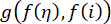 is the similarity weight of the grayscale of the centre pixel i and η represents the nearby pixel, central pixel i,q(η,i) function is the weight of the geometric similarity value and its surrounding pixels η, h(i) is the normalization index.

   (3)

Gaussian kernel function is computed to determine geometric similarity between the central pixel and surrounding pixels. The following steps were taken to construct the Gaussian image kernel function to determine geometric similarity.

   (4)

where d represents the geometric expansion factor, which primarily limits the geometric expansion factor of the low-pass filter intensity and d(η,i) stands for the distance among the surrounding pixel point η and the central pixel point i. The low-pass filtering power decreases with decreasing χ_d value, and the resulting filtering result becomes clearer. The construction of the Gaussian kernel function of grayscale similarity is as follows,

   (5)

The diffusion factor for grayscale image similarity is called χ_r. Equations (1) to (5) show that with conventional bilateral filtering, each pixel must be evaluated numerous times, resulting in the poor real-time performance of the method. Mean and standard deviation is computed for each sample within the reference window. The terms μ_w and σ_w are expressed as Equations (6-7),

   (6)

    (7)

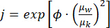
All data within the local reference frame would be kept and subjected to bilateral filtering if μ_w and σ_w  Equation (6); otherwise, the samples would be removed. After the trimming of the samples, the combined weight of filtering k(i), which is produced by Equations (5) to (7), as well as the initial sample, η is then swapped out for the trimmed sample φ. Depending on the trimming depth value j, the edge similarity index (ESI) and equivalent view number of looks (ENL) are utilized to evaluate how effectively the bilateral filter preserves the edges of an image during processing.

The ENL and ESI were computed to evaluate edge preservation and speckle reduction. ESI assesses how comparable the edge maps of the original and filtered images are, whereas ENL is calculated as  within a homogeneous image region, where larger ENL values indicate stronger speckle suppression. As the value of trimming depth increases, more sample data and image features are maintained, but despeckling efficiency will decrease. The construction of the depth kernel function is specified as Equation (8),

    (8)

where μ_k represents the value of the overall image’s standard deviation μ_w and  represents the local reference window’s standard deviation value. In the truncated image, a smaller weight value φ represents a higher ability to shorten the image feature information. The amount of automatically trimmed data samples is lower, the edge data and texture of j image are well retained, and μ_w is more than μ_k as well as the value of A is larger if the filtered pixel is an edge pixel in the image. However, if the pixels filtered are mostly cluttering pixels, μ_w is smaller than μk and smaller j becomes more pixels that diverge from the deleted images of the mean value. As a result, there are a lot of automatically trimmed samples, which can significantly improve the smoothness of the speckle noise. The significant speckle noise signal is smoothed due to the improved accuracy of the enhanced combined similarity weight, which also aids in keeping the image’s edge detail information. After the pre-processing stage, the denoised image is then given to the feature extraction stage, where the features are extracted by SIFT techniques.

Feature extraction

SIFT feature extraction is implemented with the OpenCV library, ContrastThreshold is 0.04, edgeThreshold is 10, sigma is 1.6, features are 500, and OctaveLayers is 3, which are the parameters that are set. Low-contrast and edge-response keypoints were filtered using standard SIFT criteria, and only the remaining stable keypoints were used for feature extraction. Enhancing classification performance requires feature extraction. In this work, robust features are extracted from pre-processed images using the SIFT approach. By identifying keypoints and characterizing them using 128-dimensional descriptors based on local gradient orientations, SIFT successfully manages issues including scale and rotation variations, light alterations, and perspective rotations.

Although convolutional neural networks can learn hierarchical features end-to-end, the inclusion of SIFT-based handcrafted features in the proposed framework is motivated by their ability to capture scale- and rotation-invariant local keypoint descriptors, which can be particularly helpful in situations with little data variability or subtle disease patterns. By adding robust local structure information to the learned representations, SIFT features improve the discriminative capability in the work. It is acknowledged that adding hand-crafted features to deep learning increases computing costs and may not always be necessary, especially when large and diverse datasets are available for end-to-end training. The current study employs this hybrid approach to benefit from the advantages of both paradigms, particularly when working with controlled datasets.

Extreme detection for scale in space: This phase of filtering aims to isolate the scales and locations that can be distinguished between images of the same object. The ‘scale space’s function is used to find an effective way. Furthermore, it has been demonstrated that Gaussian functions are based on probabilistic assumptions. Equation (9) defines the scale space:

    (9)

The term E(p,q,π) represents the scale space, U(p,q,π) is a variable-scale Gaussian, I(p,q) is the input image and (•) is the convolution operator.

The next step is to identify the keypoints’ stable positions in the scale space using a variety of techniques. Such a method is the variance of the Gaussians, which locates scale-space extrema, B(p,q,π) by calculating the difference among two images, where one image has a scale g times than the other image. Difference of Gaussians (DoG) computation refers to how the DoG image is calculated in the SIFT algorithm. It is obtained by subtracting two Gaussian-blurred versions of the same image at different scales. The expression for D(p,q,π) in Equation (10):

    (10)

Every theme is contrasted with 8 neighbours on the same scale, as well as 9 neighbours down and up a scale to find the local maximum and minimum values of D(p,q,π). An extrema is a point that lies between the lowest and highest values among all these points.

Localization and filtering of the key point

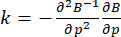
This step identifies the weak contrast images and incorrectly positioned images on the edge and eliminates the additional essential spots from the list. This computes the Laplacian value for each keypoint identified in step 1. The following Equations indicate where the extremum, k is in Equation (11):

    (11)

When the function value at k is lower than a predetermined level, this point is degraded. Low contrast extrema are eliminated in this way. As a result, extrema determined by insufficient localization are eliminated in some cases when there is a considerable principal curvature at the boundary but a tiny curvature in the opposite direction in the variation of the Gaussian function. When the variations are less than the ratio of the eigenvector from the 22 Hessian matrix at the location and scale of the key point, then it is ignored.

Assignment of orientation

Using local image attributes, this step will provide continuous orientation to the key points. Once expressed in relation to this orientation, the keypoint descriptor, which is detailed below, becomes rotation-invariant. select the Gaussian-smoothed image corresponding to the scale of the keypoint. Next, calculate the gradient magnitude, h using:

    (12)

and determine the gradient orientation, Φ using:

   (13)

Construct an orientation histogram from the sampled points and identify the highest peak. Assign the dominant orientation represented by this peak to the keypoint. Additional peaks with heights equal to at least 80% of the highest peak may also be assigned, resulting in multiple orientations for some keypoints. For each selected peak, fit a parabola to the three nearest histogram values to interpolate the peak location more accurately.

Keypoint descriptor:

Keypoint descriptors are created by applying Gaussian weighting depending on the keypoint scale and aligning the local gradient information with the keypoint orientation. Each cell in the 4 × 4 grid created by dividing the image region has an 8-bin orientation histogram. For every keypoint, a 128-dimensional feature vector is created by combining these histograms.

Feature selection

To decrease dimensionality and increase efficiency, the feature selection stage finds the most pertinent features. In this work, redundant features are removed using the COA, a population-based metaheuristic motivated by coati behavior.

The Coati Optimization Algorithm is a minimization problem where the fitness function simultaneously minimizes the classification error and decreases the number of selected features. The objective is to identify the optimal feature subset that achieves high classification accuracy while reducing feature redundancy. The fitness function is defined as follows:

  (14)

where, S represents the features subset, f represents the total feature set, α,β are the weighting factors. Initializing feature placements in the search space at random is the first step in the method.

  (15)

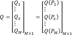
In Equation (14), P_x denotes the location of the x^th feature in the search area, p_x,y indicates the range of y^th decision variable, M denotes the number of coatis, N represents the number of decision variables, rand denotes a random number ranging between 0 and 1 and UB_y and LB_y  specifies the upper bound and lower bound of the y^th decision variable. The population initialization of COA is given in the matrix.

    (16)

where,Q mentions the discovered objective function’s vector and Q_x represents the discovery of the discovered objective function based on x^th coati. Each iteration of the algorithm updates the candidate solutions, which update the best features. The two distinct phases of updating the COA population are explained as follows.

Hunting and attack tactics (exploration phase)

In the exploration phase, search agents can migrate to different locations within the exploring region and demonstrate the COA’s ability to search globally within the problem-solving area.

Equation (17) represents the position of the best features,

  (17)

The update process will accept the new feature locations if they raise the goal function value; otherwise, the search agents will remain in their previous placements. The position updation of search agents to obtain the optimal features is expressed as,

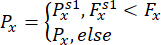   (18)

where  mentions the updated position of  x^th search agent, the objective function value is represented as . The term rand represents the random value ranges from 0 to 1. Iprey represents the feature's location in the exploring region, which refers to the best position, Iprey _y denotes the y^th position, I is an integer randomly selected among [1, 2], the location of the prey is represented as ,  is the y^thdimension,  is the objective function and (•) specifies the great integer function or floor function.

The action of fleeing predators (exploitation phase)

In the exploitation phase, the location of search agents in the exploring region is changed based on the natural behavior of each piece of information in encountering and avoiding predators.

Equations (19) and (20) are employed to analyze the random spot to mimic the behaviors of each coati.

  (19)

  (20)

The newly generated position is beneficial and is represented as Equation 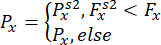(21)

   (21)

here,   indicates the objective function value, is its y^th dimension, rand is a random term varied between 0 and 1, c represents the iteration count and  and  are the local lower bound and upper bound of the y^th decision variable, respectively. The terms LB_y and UB_y mentions the lower bound and upper bound of the y^th decision variable. The basic flowchart of the optimization technique is given in Figure 2.

Classification

The suggested CA-CSSAE model is used for classification following feature selection. This hybrid architecture efficiently learns discriminative and hierarchical features by combining convolutional layers, stacked sparse autoencoders, and attention algorithms. The attention module suppresses unimportant information while highlighting significant patterns like lesions and textures. The following hyperparameters, like learning rate 0.001, batch size 64, activation tanh, epochs 300, optimizer Adam, and hidden units 2, are used to divide the tomato illnesses into 10 classes.

To improve reproducibility, the CA-CSSAE architecture has been described layer by layer, as initially Convolution Layer (3 × 3 × 3 pixels) follows Max Pooling Layer (2 × 2), then a Cross-Attention Layer. Subsequently, perform SAE1 (200 hidden units), then SAE2 (400 hidden units) follows Softmax Output Layer (10 classes), then the final image (32 × 32 × 3 pixels). The model was trained using the categorical cross-entropy loss function, and then it was optimized using Adam. The notation 32 × 32 × 155 represents a feature tensor of spatial size 32 × 32 pixels with 155 extracted feature channels. Tomato leaf sections that have already undergone background removal and noise filtering are called segmented images.

A layer of attention that has been modified for the proposed model is called the cross-attention layer. In there, N the number of CSSAE.  is the input features, where  is the input image. The terms d and p refer to the dimensions of the image and the number of pixels, respectively. The i^th CSSAE hidden output is represented by the formula   where 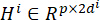,  dⁱstands for the i^th CNN hidden dimension. As indicated in the following Equation (24), the row-max-pooling is employed for j^th CSSAE hidden output, which has the form .

  (22)

where 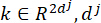represents hidden dimensions of the j^th CNN. To get query matrix K , the k is used n times where

The attention weight is then calculated using the additive approach, as stated in the following expression:

  (23)

 (24)

where, tanh function is used in this instance as the activation function. The relevance of the q^th hidden output of the j^th CNN is indicated by the expression . The weighted average representation of the hidden output of the j^th CNN is obtained using the normalized attention weight  as demonstrated in the following formula:

   (25)

where  represents the hidden dimension of the j^th CNN. The final pixel form h_s is created by combining  and   as given inside the expression below:

   (26)

where . The value of i depends on the value of j. The element from {1,2,...,j-1}, i is a subset of all sets made up of elements.

The essential building block of a CNN is the convolutional layer. Assume a convolutional layer now where the convolution kernel is E_N×N and the input is a matrix L_M×M in which the padding is 0, and the stride is 1. This layer’s output is C of size (M - N + 1)×(M - N +1), and Equation (29) shows how to estimate C.

   (27)

where ReLU, Leaky ReLU, or Sigmoid are examples of non-linear activations f. The pooling layer, which is commonly max pooling or average pooling, is a further basic building block in CNN. By reducing the output size, the pooling layer could further minimize the computing complexity.

Unsupervised learning is the foundation of AE neural system functions (feed-forward back-propagation). The input images are reconstructed using AE, which produces same sized output images. The encoder and decoder phases are the two important processes in the AE model. Assume a vector X contains unlabelled sub-inputs, which are represented by the letters

The Z hidden layers  that are produced during the encoder stage are shown in Equation (30).

  (28)

The kernel vector and bias are represented by a and b respectively. The activation module’s symbol is . (As defined in Equation (31)).

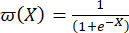   (29)

The reconstruction or decoding phase is indicated by Equation (30).

   (30)

where represents the reconstructed vector’s result, a represents the kernel vector, b mentions the bias value and  represents the error value introduced during back-propagation.

At the hidden layer Z, the stacked autoencoder (SAE) has sparsity parameters. The main objective of SAE is to quantify the ideal kernel values (a,a) and associated bias representations (b,b). Then, as shown in Equation (31), the optimal values are obtained by minimizing a cost function.

   (31)

where ε is used to represent the MSRE (as shown in Equation (32)).

   (32)

here γ stands for the weight decay module (also called the L2 regularisation weight). This reduces overfitting (which is mentioned in Equation (31)).

   (33)

where η (controls weight), as mentioned in Equation (33) and  shows the sparsity penalty (sparsity regularization)

(34)

where λ indicates the value of the sparsity parameter. l_n mentions the entire number of neurons in the hidden layer, while KI stands for the KL (Kullback-Leibler) divergence unit. The average activation values of the hidden neurons are given as .

Layers SAE1 and SAE2 are stacked to reduce the dimensionality of large feature maps. The first SAE output serves as the second SAE’s input. As the innermost layer of the stack, shallow SAE is used rather than the entire SAE. The term “Shallow SAE” refers to the SAE-exclusive encoder section that has been chosen for the process of feature learning and acquisition. The features are also passed on to the following layer. The softmax is chosen to connect the layered network.

   (35)

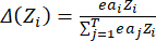   (36)

where z_i is used to represent the CA-CSSAE output. Classification based on probability is done using the softmax classifier Δ. With T  showing all classes, a_i stands for the i^thneuron unit kernel vector. The probability of the i^th class is displayed in the output Δ(Z_i).

For training the CA-CSSAE, the segmented images (X) are provided. There are 155 slices in the input vector, which has a size of 32 × 32 × 155. As a result of the input 32 × 32, the CA-CSSAE model is given 1024 units. It is sent to SAE1 as an input with 200 concealed units. An initial image vector is constructed in SAE1 with bias and weight, and then it is fed into SAE2 as an input. In SAE2, a feature vector is produced using 400 hidden units together with bias, weight and many hyperparameters. On the basis of the feature vector acquired from SAE2, the classification is performed using the softmax layer. Also, the parameters of the proposed CA-CSSAE model are fine-tuned by using the Adam optimizer to mitigate the training complexities. Figure 3 represents the classification model of the proposed model.

Experimental analysis

The proposed work is implemented in a Python tool, with Python libraries used in the implementation including TensorFlow, Keras, OpenCV, NumPy, SciPy, Scikit-learn, and Pandas, with the PlantVillage dataset. The computer was equipped with a 64-bit operating system, an x64-based processor, an Intel Core i5-3470 CPU running at 3.20GHz and 8GB of installed RAM. The proposed model is evaluated with existing models for key elements like accuracy, precision, recall and f-measures. The research compared many plant diseases like LB, YLCV, BS, EB, TSSM, TMV, LM, SLS and TS. A detailed explanation is given in the following section.

The COA's stopping criterion is set at a maximum of 100 iterations or until the fitness improvement set at 10^-4 convergence threshold. The COA population has thirty agents. For model initialization, Xavier (Glorot) initialization is used for convolutional and autoencoder weights, and biases are initialized to zero. Every test uses a predetermined random seed value of 42 to ensure reliable and reproducible results. A batch size of 64 and a learning rate of 0.001 are used during 300 epochs of training. The 2 hidden units is the number of hidden layers in the architecture. After evaluating several settings, the optimal trade-off between computational efficiency and model performance was found in the selected setup. The hyperparameter tuning was performed using manual trial-and-error.

It was discovered that a reduced number of hidden units was adequate to avoid overfitting and computational overhead while simultaneously capturing the key feature representations following dimensionality reduction via COA. These requirements offer experimental consistency and greatly improve the suggested procedure's repeatability, transparency, and dependability. Table 1 displays Reproducibility and Implementation Settings.

The implementation settings utilized in this investigation to guarantee reproducibility are summarized in Table 1. By clearly defining these parameters, the suggested model's transparency and dependability are increased, and consistent experimental replication is made possible.

Dataset details

The PlantVillage dataset, a publicly available standard dataset for categorizing plant diseases, was used in this study. There are about 54,000 images of plant leaves from 14 distinct crop varieties, both healthy and diseased. From this dataset, only the tomato leaf subset, which comprised 20,732 images of both healthy leaves and different tomato disease categories, was selected. Every image has a resolution of 250 × 250 pixels. Before feature extraction, the recommended Adaptive Threshold-Based Bilateral Filtering technique was applied as a preprocessing step to enhance image quality and reduce noise. The selected tomato photographs were divided into training, validation, and testing sets using a 70:20:10 ratio. From this, the proposed study has chosen the tomato crop, which is presented in a separate folder²⁶. The resolution of each image in this dataset is 250 × 250 pixels. Table 2 represents the total number of images of the diseases present in the tomato plant.

結果

Performance evaluation for different types of disease

The proposed model is evaluated using different diseases in terms of accuracy. The proposed model achieved an accuracy value of 99.87% for EB, 99.1% for LB and 99.23% for TMV, respectively. Furthermore, the existing methods reproduced and evaluated each current strategy under the same experimental conditions, such as the same dataset, data split, evaluation metrics and hardware/software environment, to provide a fair and objective comparison. The existing methods achieved an accuracy of 99.88% for HL, 99.69% for LM and 99.74% for YLCV, respectively. The value of BS is 99.44%, with a score of 99.5% for SLS and TMV of 99.3%, including 99.31% for SM disease. The proposed model achieved the best values for all diseases, as shown in Figure 4. The results are multiple runs with averaged values. A more reliable, consistent, and impartial evaluation of the performance of the proposed model is produced by averaging the results, which lessens the effects of random initialization, stochastic optimization, and data variability. The proposed approach ensures that the given metrics are representative rather than depending on a single trial result. Figure 5 illustrates the accuracy and loss attained by the proposed model during the training, testing and validation process.

Performance evaluation using various models

Models like DenseNet (DN), GNN, MobileNet (MN), a combination of SqueezeNet and AlexNet (CSA), Inception V3 (IV3), VGG-16, and DCNN are compared with the proposed model. Comparative models were evaluated using the same dataset subset, split ratio, pre-processing, and training conditions. The comparison values from this study in terms of overall accuracy, the DN achieved 97.25%, the GNN achieved 95.1%, and the MN attained 91.2%. The CSA has a 90.3% accuracy rate, while IV3 has the lowest (63.4%). The VGG-16 achieves 77.2% accuracy, while the proposed model achieves 99.5%. The proposed model has a clear edge over other models in terms of accuracy, which is illustrated in Figure 6.

The f-measures of the proposed and Deep neural network (DNN) are given in Figure 7. In terms of disease classes, the proposed model is compared with the Deep convolutional neural network (DCNN) model, in which the DCNN model achieved an F-measure of 0.95 in terms of EB and 1 for LB disease. The DCNN achieved 0.96 of f-measure value for TMV and managed to score 0.97 and 0.98 in terms of HL and LM, respectively. The DCNN scores 0.96 for YLCV and has scores of 1 and 0.98 for BS and SLS. The existing model scores 0.94 in TS and 0.99 for SM, respectively. The proposed model scores 0.98 in terms of EB, 0.99 for LB, 0.99 for TMV, 1 for HL, 0.99 for LM, 0.99 for YLCV, 0.99 for BS, 1 and 0.99 for SLS and TS and scores 0.99 for SM. The class-wise comparison of the DCNN and the proposed model is given in Figure 7.

The existing model has a precision value of 93% for EB, 96% of precision for LB, 97% for TMV, 96% for HL, 93% for LM and 94% for YLCV, respectively. The BS of the existing DNN method is 96%, along with 96% of SLS, 96% of TS, and 96% of SM. The proposed model achieved the value of 98% of EB, 99% of LB, 98% of TMV, 99% of HL, 99% of LM, 99% of YLCV, 99% of BS, 98% of SLS, 99% of TS and SM has the value of 99%, respectively. Figure 8 shows the precision of the proposed and existing models in various disease classes under the same dataset split and pre-processing conditions.

A recall of the proposed model and the existing model is given in Figure 9. Recall values are computed on the test set only. The existing model has a recall value of 95% in Early Blight (EB), 99% for Late Blight (LB), 99% for Tomato Mosaic Virus (TMV), 97% for Healthy Leaves (HL), 95% for Leaf Mold (LM), 93% for Tomato Yellow Leaf Curl Virus (YLCV), 99% in Bacterial Spot (BS), 96% in Septoria Leaf Spot (SLS), 94% of Target Spot (TS) and 98% of Spider Mites (SM) respectively. The proposed model achieved the recall values of 98% in EB, 99% in LB, 99% for TMV and 99% in HL, respectively. Furthermore, the proposed model achieved 99% for LM, 97% for YLCV, 99% for BS, 99% for SLS, 98% for TS and 98% for SM, respectively. The confusion matrix of the proposed model corresponding to the test set is given in Figure 10.

The results presented in this study are based on a 70:20:10 training, testing, and validation split, which might not adequately represent the stability and variability of the suggested model. The robustness of the claimed performance is limited by the lack of repeated experimental runs and statistical metrics like standard deviation or confidence intervals. Future research will include multiple independent runs using various random initializations and data splits to overcome this limitation. To provide a more accurate assessment of model generalization, 5-fold cross-validation will also be taken into consideration. The validity of the experimental results will be strengthened by including these statistical analyses, which will provide a more thorough, dependable, and repeatable examination. Table 3 provides the statistical confirmation of the suggested model's performance.

The PlantVillage dataset, which comprises lab-controlled photos, is the only dataset used in the current study to test the model. Background complexity, illumination variability, noise, and leaf occlusions change significantly between controlled datasets and real-world field circumstances, as Table 4 summarizes. When used in real-world agricultural settings, these variables may cause a distribution shift that lowers model performance. Therefore, even though the suggested model achieves great accuracy in controlled environments, its robustness and capacity for generalization still need to be thoroughly verified. Future work will evaluate the proposed method's performance under different conditions using real-world datasets and cross-dataset assessments to enhance its dependability and utility. Table 4 presents a comparison between the controlled dataset and real-world settings.

Ablation study analysis

Each method generated in this study effectively performs on the CA-CSSAE model to obtain improved accuracy results while categorizing multiple tomato diseases. In this, the accuracy result of the proposed CA-CSSAE model without the presence of pre-processing using ATBF. The performance of the proposed model without utilizing the feature extraction step. Also, the feature selection stage and the accuracy result of the proposed CA-CSSAE model are evaluated. Accuracy is calculated by neglecting convolutional layers in the CA-CSSAE model. The result of the proposed model, including all steps. The hyperparameter sensitivity analysis is given in Table 5. Table 6 illustrates the accuracy of the result evaluation in the ablation experiment.

Ablation study analysis is provided in Table 6, which shows that model elements and parameter settings have a substantial impact on performance, with the best combinations yielding the maximum accuracy.

Computational complexity analysis

The computational complexity of the suggested CA-CSSAE framework is cumulative over several stages and input-dependent. In particular, the complexity introduced by ATBF and SIFT during the feature extraction phase is O(N .d) roughly represented by the number of input pixels N and the feature dimension d , respectively. The number of iterations D , population size P, and feature dimension I , respectively, are shown by the iterative cost of the feature optimization step O(I.P.D) using COA. With convolutional complexity increasing as O(H.W.K².C_in,C_out) and attention mechanisms scaling as O(N² .d), the classification stage, which combines convolutional operations and cross-attention mechanisms, adds even more computing overhead. Furthermore, the complexity introduced by the stacked sparse autoencoder is often proportional to the number of layers and neurons, typically O(L .n²).

Additionally, the suggested protocol uses a composite pipeline (ATBF + SIFT + COA + CA-CSSAE), which offers trade-offs in terms of computational complexity, module dependencies, and higher processing latency, even though it improves feature quality and classification accuracy. The staged architecture may result in repetitive computations and limited global optimization, in contrast to end-to-end deep learning models that jointly optimize feature extraction and classification. These reasons may hamper scalability and real-time deployment in resource-constrained contexts. As a result, even though the suggested method performs better, its complexity is best described as polynomial and multi-stage, underscoring the need for further research on model simplification, end-to-end learning integration, and lightweight deployment techniques.

Overall, the proposed CA-CSSAE framework consistently outperformed the compared methods across all evaluation metrics on the PlantVillage dataset. The ablation study demonstrated that each component contributed to the overall performance, while the computational complexity analysis highlighted the trade-offs associated with the hybrid architecture. These findings support the effectiveness of the proposed framework for accurate tomato disease classification under the evaluated experimental conditions.

DATA AVAILABILITY:

This study made use of the publicly available PlantVillage dataset. There are 54,000 plant leaf images from 14 distinct crop varieties, both healthy and diseased. The 20,732-image tomato leaf subset was supplied by the PlantVillage repository and is accessible to the public through the Kaggle platform and the PlantVillage project website. The dataset link is https://www.kaggle.com/datasets/abdallahalidev/plantvillage-dataset. Since the study makes use of a publicly accessible dataset, the scientific community already has unlimited access to all raw picture data. No new proprietary data was obtained from this research.

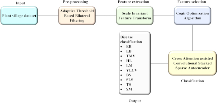
Figure 1: Workflow of proposed system. illustrates the full processing pipeline, including picture preprocessing, feature extraction, feature selection, and sickness classification, using the proposed CA-CSSAE framework. Please click here to view a larger version of this figure.

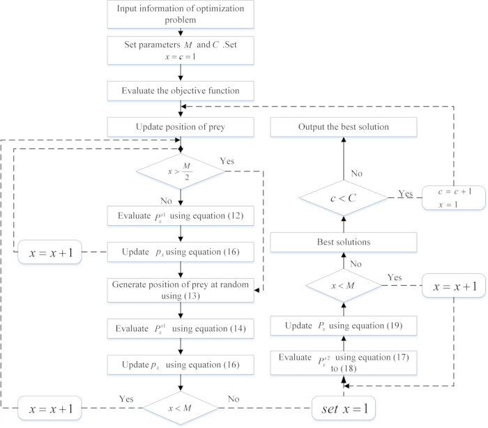
Figure 2: Basic flowchart of the proposed COA. illustrates the Coati Optimization Algorithm's phases for population initialization, feature subset optimization, fitness evaluation, exploration, exploitation, and convergence. Please click here to view a larger version of this figure.

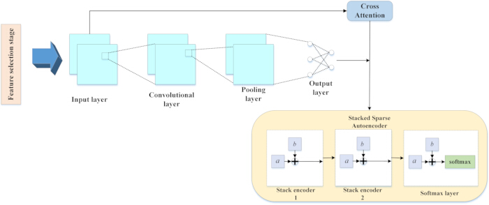
Figure 3: Classification module of the proposed model. demonstrates the Cross-Attention Aided Convolutional Stacked Sparse Autoencoder (CA-CSSAE) architecture's feature fusion, sparse representation learning, and final sickness classification. Please click here to view a larger version of this figure.

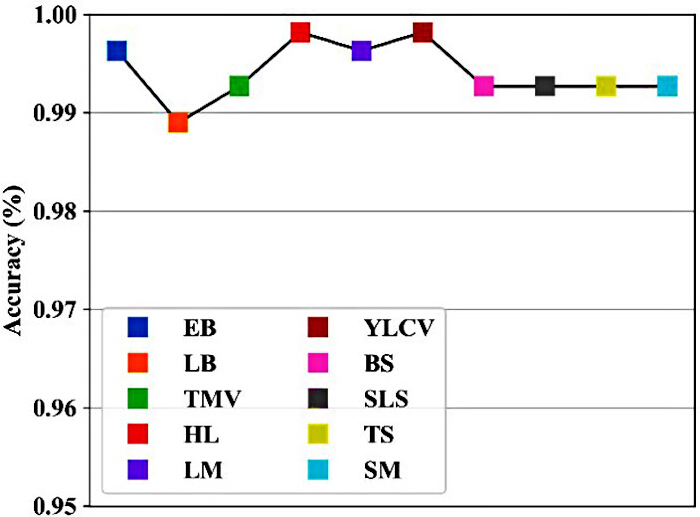
Figure 4: Overall accuracy of each disease from testing sets. demonstrates the model's performance across various disease categories by displaying the classification accuracy attained for each tomato disease class. Please click here to view a larger version of this figure.

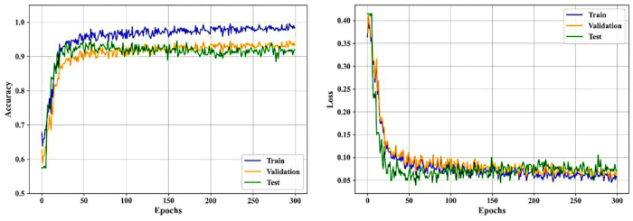
Figure 5: Accuracy and loss analysis of the proposed model for varying epochs from test sets. shows how accuracy and loss have changed across several epochs, demonstrating training convergence and persistent learning behavior. Please click here to view a larger version of this figure.

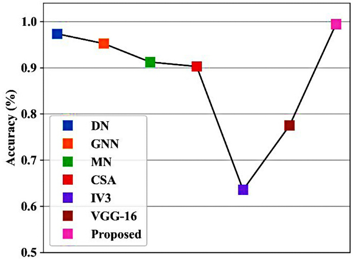
Figure 6: Overall accuracy of the proposed model with testing data. assesses the overall classification accuracy of the suggested CA-CSSAE model using the test dataset. Please click here to view a larger version of this figure.

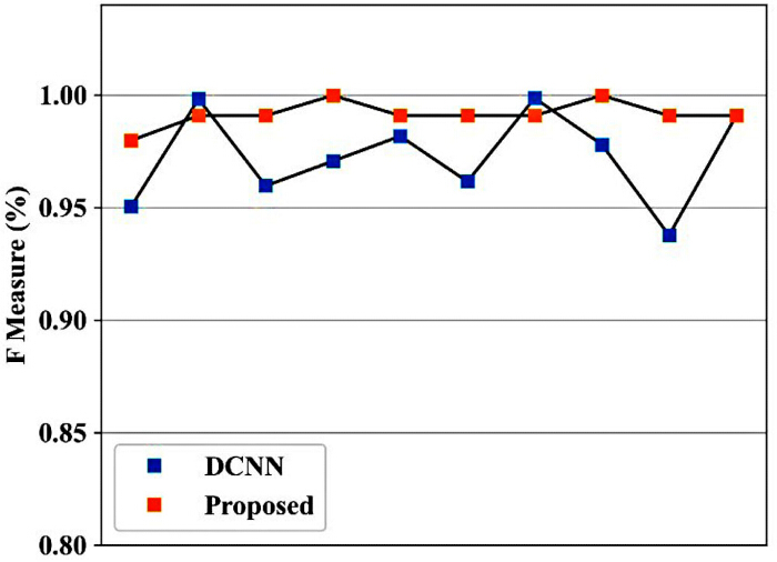
Figure 7: F-measure comparison of the DNN and proposed model with testing data. demonstrates gains in balanced classification performance by contrasting the proposed model's F-measure values with the baseline DNN's. Please click here to view a larger version of this figure.

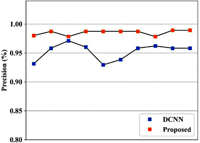
Figure 8: Precision comparison for existing and proposed models with testing data. demonstrates the effectiveness of the proposed framework in identifying diseased tomato leaves by contrasting the recall values obtained by different models. Please click here to view a larger version of this figure.

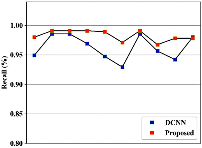
Figure 9: Recall of the proposed and existing models with testing data. demonstrates the effectiveness of the proposed framework in identifying diseased tomato leaves by contrasting the recall values obtained by different models. Please click here to view a larger version of this figure.

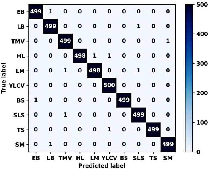
Figure 10: Confusion matrix. demonstrates the classification accuracy by displaying the distribution of samples that were correctly and incorrectly classified as well as the expected and actual illness classes. Please click here to view a larger version of this figure.

Component	Parameter	Value
Initialization	Weight Initialization	Xavier (Glorot)
	Bias Initialization	0
COA Optimization	Max Iterations	100
	Convergence Threshold	1 × 10⁻4
	Population Size	50
Training	Learning Rate	0.0005
	Epochs	300
	Hidden units	2
	Batch Size	64
	ATBF threshold	0.5
	Optimizer	Adam
Random Control	Random Seed	42
Model	Attention Heads	8
	Embedding Dimension	256

Table 1: Implementation Settings and Reproducibility. outlines the equipment, software, parameter settings, and implementation details required to duplicate the recommended process.

Disease	Number of images
TMV	2190
YLCV	1802
TS	2270
LB	1800
HL	1600
BS	2380
SM	2340
EB	2250
LM	2000
SLS	2100
Total	20732

Table 2: Different types of diseases and the number of images. highlights the various types of diseased images in the PlantVillage dataset and number of Images.

Metric	Fold 2	Fold 3	Fold 4	Fold 5	Mean ± Standard deviation	t-value	p-value	95% Confidence interval (%)
Accuracy (%)	99.5	99.4	99.6	99.5	99.46 ± 0.11	4.82	0.003	99.31–99.61
F-Measure (%)	99.1	99	99.2	99.1	99.06 ± 0.11	4.35	0.005	98.93–99.22
Recall (%)	99	99.1	99.2	99	99.02 ± 0.13	3.98	0.007	98.86–99.18
Precision (%)	99.1	99	99.2	99.1	99.06 ± 0.11	4.27	0.005	98.92–99.20

Table 3: Preliminary Statistical Validation of Proposed Model's Performance. shows the model's consistency by presenting performance data obtained over multiple experimental runs, such as the mean accuracy and standard deviation.

Stages	Controlled Dataset (PlantVillage)	Real-World Field Conditions	Performance of the Proposed Model
Image Acquisition	Recorded in a lab environment	Captured in unchanged agricultural settings	99.5% on the controlled dataset, 93% on the field dataset
Noise	Very little or no sound	Sensor noise and blur are present	High resilience, noise induced decline
Illumination	Regular lighting conditions	Variable illumination, including shadows and sunshine	Stable, decreased performance
Model Performance	Exceptionally high precision (99%–100%)	Possible decline in performance	95% on the field dataset and 99.5% on the controlled dataset
Leaf Position	Separated and easily observable	Partially obscured, overlapping leaves	Precise, but less precise when obscured
Variability	Minimal variation within the class	Significant variation in the manifestation of diseases	Robust, generalization decline
Dataset Bias	Elevated	Low	A small risk of overfitting in a controlled dataset
Evaluation Strategy	Evaluation of a single dataset	Field testing and cross dataset analysis are necessary	Additional validation is required for practical implementation

Table 4: Comparison between controlled dataset and real-world settings. highlights factors that may affect model deployment by drawing attention to the differences between the controlled PlantVillage dataset and real-world field conditions.

Parameter	Values Tested	Accuracy (%)
ATBF Threshold	0.2	95.8
ATBF Threshold	0.5	97.6
ATBF Threshold	0.8	96.9
Embedding Dimension (d)	64	97.5
Embedding Dimension (d)	128	98.9
Embedding Dimension (d)	256.0000	99.5
COA Population Size (P)	10	96.8
COA Population Size (P)	30	98.9
COA Population Size (P)	50	99.5
Learning Rate	0.001	98.2
Learning Rate	0.0005	99.5
Learning Rate	0.0001	98.7
COA Iterations (I)	20	96.2
COA Iterations (I)	50	98.4
COA Iterations (I)	100	99.5
Attention Heads	2	97.2
Attention Heads	4	98.8
Attention Heads	8	99.5

Table 5: Hyperparameter Sensitivity Analysis. evaluates the effects of different hyperparameter changes on model performance to identify the configuration that produces the best results.

Model components	Precision (%)	F1-Score (%)	Accuracy (%)	Recall (%)
Proposed (No component removed)	99.06	99.06	99.46	99.02
Preprocessing module removed	98.51	98.47	98.72	98.43
Feature fusion module removed	98.36	98.32	98.54	98.29
Attention module removed	98.65	98.62	98.87	98.59
Feature extraction module removed	98.12	98.08	98.31	98.05
classification removed	98.8400	98.81	99.02	98.78

Table 6: Ablation Study analysis. assesses the model's performance following the removal or modification of modules to demonstrate the contribution of each key element of the proposed framework.

ディスカッション

The proposed CA-CSSAE model demonstrates strong performance in tomato disease classification, achieving high accuracy, precision, recall, and F-measure across several disease classes with test data. Each component, such as pre-processing (ATBF), feature extraction (SIFT), feature selection (COA), and classification (cross-attention with stacked sparse autoencoder)²¹, contributes positively to overall performance, according to the ablation study. Specifically, the complete model configuration attains 99.5% accuracy, demonstrating the efficacy of combining several phases for improved feature representation and classification. Nevertheless, several restrictions must be noted in spite of these encouraging outcomes. Only the PlantVillage dataset, consisting of laboratory-controlled images, is used to validate the model²⁶. This limits the model's applicability to real-world agricultural settings, where factors such as noise, occlusions, complex backgrounds, and fluctuating lighting are common. The multi-stage composite pipeline used in the suggested approach increases computational complexity and may restrict its use in real-time or resource-constrained scenarios. The model's scalability depends on several factors, including input size, attention configuration, and optimization iterations, and the computational complexity analysis in the initial formulation was insufficiently precise. Furthermore, because based on a single data split without repeated runs or variance reporting, statistical validation is constrained. Lastly, to ensure fairness, comparisons were performed under identical conditions only.

This study discusses the proposed CA-CSSAE architecture, its improvements in automated tomato disease diagnosis, and its potential applications in precision farming and intelligent crop monitoring. The study's shortcomings, including its reliance on a controlled dataset and single-run evaluation, have also been identified. Alternative approaches, such as Vision Transformers, end-to-end convolutional neural networks, and other hybrid deep learning models, are discussed as potential avenues for future research. Furthermore, future work will focus on robustness analysis, validation using real-field datasets, and implementation in real-time agricultural systems^19,20.

To determine the model's resilience in a variety of environmental circumstances, it will be tested on real-world datasets and validated across multiple datasets. Variants of the model that are computationally efficient and lightweight for deployment on edge devices will be developed. A thorough hyperparameter sensitivity study using automated tuning techniques such as grid search or Bayesian optimization will also be part of future work. To decrease pipeline complexity and increase scalability, the integration of end-to-end deep learning architectures will also be investigated. To ensure the accuracy of the results, a preliminary statistical validation is performed in Table 3. These enhancements will increase the suggested approach's capacity for generalization, reproducibility, and practical application.

This study proposed a hybrid deep learning model that reduces the errors and limitations of prior methods. Initially, the images are pre-processed to improve the quality of raw inputs. Then, the relevant features are extracted and selected using efficient methods. The proposed CA-CSSAE model categorized multiple tomato leaf diseases, including EB, LB, TMV, HL, LM, YLCV, BS, SLS, TS and SM²⁶. The results show that the proposed model achieves an improved accuracy of 99.5% and outperforms existing methods. However, the proposed work does not analyze the model interpretability of the CA-CSSAE model, and this work does not include real-time evaluation. Therefore, in the future, the proposed study will be extended by utilizing an explainable AI method for interpreting the model’s ability in the feature learning process. In addition, a robust feature extraction method can be used in the future to handle real-time data scenarios and evaluate the efficacy of the proposed model in complex environments like varied soil types and lighting conditions^22,23. SIFT-based feature extraction, which produces handcrafted features that are invariant to rotation and scaling, is used in the current study. However, more advanced and adaptable feature extraction methods, such as deep learning-based feature representations that can automatically extract discriminative features from real-time field photographs, will be the focus of future study. These techniques should be more robust to variations in illumination, soil backdrops, occlusions, and environmental complexity than the current SIFT-based method²¹. Moreover, lightweight architectures will be designed in the future to maintain computational efficiency for resource-constrained devices. Also, future work will be improved by analyzing diseases in other plants, such as potatoes, rice, and peppers. The practical implications of tomato leaf disease categorization for the agriculture sector are substantial. Automatic disease identification can reduce the necessity for manual inspection and labour costs. Also, to create a comprehensive crop management process, the model can be combined with drone- or IoT-based devices.

材料

この記事で使用された材料の一覧

名前	会社	カタログ番号	コメント
Deep learning framework	Google LLC	Version 2.x, https://www.tensorflow	TensorFlow
Operating System	Custom built system	x64-based architecture	64-bit Operating System
Processor	Intel Corporation	https://www.intel.com	i5-3470@ 3.20 GHz;  Intel Core i5-3470 CPU @ 3.20 GHz
Programming Language	Python software foundation	Version 3.x, https://www.python.org	Python
RAM	Generic/OEM	/	8 GB DDR3 RAM