マウスモデルは、胚発生の理解を深める上で極めて重要な役割を果たしています。本稿では、固定されたマウス胚全体のタンパク質および転写物を染色するためのプロトコルと、得られた染色結果を3次元的に定量分析する方法について説明します。これらの手法を用いることで、発生における主要な細胞型やプロセスの可視化および分析が可能になります。
方法論記事
マウス胚全装標本におけるタンパク質および転写産物の発生過程での発現解析の最適化手法
100 回視聴
⸱
2026年9月11日
この記事について
サマリー
要約
マウスモデルは、胚発生の理解を深める上で重要な役割を果たしてきました。胚内におけるタンパク質および転写産物の発現と局在を解析することは、発生および疾患の根底にある細胞および分子メカニズムを解明するために不可欠です。しかし、マウス胚の転写産物やタンパク質の解析に用いられる従来の技術には限界があります。RNA in situ ハイブリダイゼーションでは、転写産物のホールマウント染色が可能ですが、マルチプレックス能力に欠けています。対照的に、胚の切片作成ではマルチプレックスの標的染色が可能ですが、2次元(2D)での解析に限定されます。より最近では、RNAscopeや免疫蛍光染色などの技術がホールマウント胚に適用され、3次元(3D)での標的のマルチプレックス解析が可能になりました。これらの手法により、従来の技術による制限を受けることなく、胚発生に必要な主要な相互作用、パスウェイ、および細胞型のマッピングが可能になります。
本資料では、RNAscopeまたは免疫蛍光法を用いた、固定済み胚齢(E)8.5およびE9.5マウス胚のホールマウント染色の最適化手法について解説します。どちらの手法においても、単一の胚で最大4つのターゲットを同時にマルチプレックス検出することが可能です。また、同一胚内で免疫蛍光染色とRNAscopeを組み合わせることで、発生過程におけるタンパク質と転写産物の相互作用を可視化する方法についても提示します。さらに、Zeiss Arivis Proソフトウェアを用いて、胚全体および特定の発生段階の細胞タイプにおけるターゲット発現の共焦点イメージングおよび3D解析を行うパイプラインについて説明します。これらの手法を併用することで、マルチプレックス化したタンパク質および転写産物ターゲットの包括的な3D解析が可能となり、発生初期から中期にかけての細胞および分子レベルの相互作用を解明するための強力なシステムを提供します。
概要
マウスモデルは、マウスとヒトの発生の相同性、およびCre-LoxPやCRISPR/Cas9などの主要な技術を用いて遺伝子発現を調節できる能力により、ヒトに関連する発生プロセスをin vivoで理解することを可能にし、発生生物学の進歩に不可欠な役割を果たしてきました1,2。ゲノム領域の約90%がマウスとヒトの間で保存されており3、マウスとヒトは多くの発生プロセスを共有しています。例えば、マウスとヒトはどちらも、接合子の形成から胚盤胞への進展、それに続く着床および原腸陥入を含む、同様の胚発生のタイムラインを辿ります4。さらに、ほとんどの器官の発生はマウスとヒトで同様です。例えば、ヒトとマウスの心臓はどちらも、心ループ形成、心房および心室の中隔形成、弁形成、そして流出路形成という同様のシーケンスを経て、四心室心臓を形成します5。したがって、発生過程および完全に発達したマウスとヒトの心臓は、どちらも構造的に高い類似性を持っています6,7。
正常および病理学的な発生過程で起こる現象を調査するために、主要なタンパク質や転写産物を空間的に可視化できる複数の手法が開発されてきました。このような手法には、免疫蛍光染色やRNA in situ ハイブリダイゼーションが含まれます。
RNA in situ ハイブリダイゼーションは、1969年にGallとPardue8、およびJohn、Brinstall、Jones9によって、また1970年にBuongiorno-NardelliとAmaldi10によって初めて報告されました。本手法は、組織内における転写産物の発現を調べるために用いられます8。簡潔に述べると、目的のターゲットに対する相補的なRNA配列を含むプローブを選択し、検出用のマーカーで標識します。このような標識には、放射性標識、ビオチン、またはジゴキシゲニンが用いられます。固定した試料を透過処理してプローブを浸透させ、次いでプローブを組織にハイブリダイズさせます。その後、放射性標識した場合は直接イメージングを行い、それ以外の場合はアルカリフォスファターゼや蛍光色素を結合させた抗体を用いて標識を可視化します。RNA in situ ハイブリダイゼーションは、ホールマウント試料を染色して3D局在を解析できるという利点があります11。しかし、非常に特定の用途に最適化された手法を用いるか、あるいは染色体の蛍光標識に用いられるM-FISHのようなDNAハイブリダイゼーションを用いる場合を除き、通常は2つ以上のターゲットを同時に検出するマルチプレックス能が欠如しているという制限があります12,13。
免疫蛍光法は、1941年にCoonsらによって初めて開発されました。14,15は、固定または凍結された試料における標的タンパク質の検出法である。簡潔に述べると、試料を 組織の非標的領域への非特異的結合を減少させるため、ブロッキングを行います。その後、標的抗原に特異的な一次抗体を試料とともにインキュベートします。一次抗体は、蛍光色素やタンパク質に直接結合させておくこともできますし、一次抗体を産生させた動物種を標的とする蛍光標識二次抗体を用いて標的化することも可能です。直接標識した一次抗体よりも二次抗体を使用する利点は、シグナルが増幅され、感度が向上することです。異なる動物種で産生された複数の一次抗体を用い、直接標識抗体または異なる励起・蛍光スペクトルを持つ蛍光色素で標識した二次抗体を使用することで、標的検出のマルチプレックス化が可能です。
RNA in situ ハイブリダイゼーションや免疫蛍光染色などの従来の手法には限界があります。通常、RNA in situ ハイブリダイゼーションではサンプル内で単一の標的しか検出できないため、異なる細胞型や経路間の相互作用の解析は極めて限定的です。さらに、免疫蛍光染色は従来、ホールマウントではなく組織切片で行われてきたため、空間分解能が2Dに制限されていました。近年の手法では、3Dシステムにおける標的検出のマルチプレックス化に焦点が当てられています。免疫蛍光染色プロトコルの最適化により、本手法をホールマウントに適用することが可能になりました16。さらに、免疫蛍光染色と同様に蛍光標識プローブを用いることで、転写物の検出をマルチプレックス化する技術が開発されています。
RNAscopeは、2012年にWangらによって初めて報告されました。これは、固定サンプル内での転写産物の空間的な同定を可能にするRNA in situ ハイブリダイゼーション技術17に基づいています。簡潔に述べると、固定サンプルを透過処理し、相補的な転写産物配列に結合するターゲットプローブを浸透させます。RNAscopeプローブは、「ダブルZ設計」となっており、ターゲットRNAの18–25塩基対の領域に特異的な領域、14塩基対を含むテイル領域、および2つの「Zプローブ」を連結するスペーサー領域で構成されています。2つのテイル領域は合わせて28bpの領域を形成し、ここにプレアンプリファイアが結合します。結合したZプローブペアは、その後、プレアンプリファイア上の部位に結合する一連のアンプリファイアの結合を通じて増幅されます。アンプリファイアは、蛍光マーカーまたは西洋ワサビペルオキシダーゼ(HRP)で標識されたプローブを用いて特異的に標的化できます。プローブのダブルZ設計の意図は、未結合プローブの増幅を防いで非特異的な増幅を減少させることであり、一方で複数のアンプリファイアを使用するのは感度を高めるためです。従来のRNA in situ ハイブリダイゼーションに対するRNAscopeの利点は、ターゲットごとに異なる蛍光マーカーを使用することで、単一のサンプル内で転写産物検出をマルチプレックス化できる点にあります。RNAscopeは、サンプルのホルマリン固定パラフィン包埋切片で広く利用されており、2次元での空間的な転写産物検出を可能にしています18。より最近の研究では、マウス胚におけるホールマウントRNAscope染色の手法が報告されており、主要な発生プロセスの3次元解析が可能となっています19。
ここでは、RNAscope in situ ハイブリダイゼーションと免疫蛍光染色を併用した、固定済みE8.5およびE9.5マウス胚のホールマウント染色の最適化された手法について説明します。本プロトコルでは、E8.5/E9.5胚のホールマウントに有効な、免疫蛍光染色とRNAscopeを組み合わせた改訂手法について述べます。また、Opal 780蛍光色素を用いた4番目のRNAscopeプローブによる染色を組み込むことで、ホールマウントRNAscope染色にさらなるチャンネルを追加する方法、および染色済み胚の解析に広く適用可能な手法について詳述します。これらの手法を用いることで、免疫蛍光染色とRNAscopeによる最大4つのタンパク質および転写産物ターゲットのマルチプレックス可視化と、発生過程におけるE8.5/E9.5マウス胚のホールマウントでの定量的3D解析が可能となり、細胞移動やシグナル伝達経路などの重要な発生プロセスの知見をさらに深めることができます。
プロトコル
All animal experiments were performed in compliance with the UK Animals (Scientific Procedures) Act 1986 and approved by the University of Oxford animal welfare review board and the Home Office (Project license PP7967396).
1. Dissection, dehydration, and storage of E8.5 and E9.5 mouse embryos
- Cull pregnant females using an approved method at E8.5 or E9.5 gestation.
NOTE: Mice in this study were culled using cervical dislocation followed by confirmation of death by exsanguination. Exsanguination is performed by making an incision in the ventricles, facilitating bleeding. Other methods, such as CO2 inhalation, may be used, but were not tested in this protocol. - Open the abdomen first by cutting through the skin, then the abdominal wall.
NOTE: Swab mice with 70% ethanol to reduce dander and bacterial contamination. When opening the abdominal wall, it is important to pull the wall away from the abdomen, then make a small incision. Cut the abdominal wall in a V-shape, avoiding inadvertently cutting the uterus. - Remove the uterus by cutting where the uterus meets the vagina. For both uterine horns, cut the uterus away from the abdominal fat, making small excisions until you reach the ovary.
NOTE: It is worthwhile to make a note of the position of each embryo within the uterus. Dissect out the ovary with the uterus to help maintain orientation. - Individually cut a single embryo from the uterine horn, within the surrounding uterus, and place it in a dish containing 1× Hanks’ Basic Salt Solution with 5mM EDTA.
- Using fine forceps, gently peel away the uterus from the embryo, placenta, and the decidua surrounding the two.
- Identify where the placenta meets the part of the maternal decidua surrounding the embryo; there should be a slight difference in color between these two sections. Carefully separate the embryo by cutting through the maternal decidua to disconnect the placenta and reveal the embryo.
- Gently tease the embryo within its yolk sac from the remaining tissue. Using fine forceps, remove the yolk sac surrounding the embryo. Remove the amnion. Count somites to determine the exact embryonic stage.
NOTE: The yolk sac surrounds the embryo and is thicker and more opaque. The amnion is thin, transparent, and clings tightly to the embryo. This needs to be carefully removed to ensure downstream probe/antibody penetration. For older embryos, a hole can be poked in the head with fine forceps to prevent probe trapping in the developing brain ventricles. It is important at this point to remove as much of the yolk sac as possible. Leftover yolk sac fluoresces strongly when anti-mouse secondary antibodies are used. - Optional: Store the yolk sac for genotyping by washing in 500 µL of PBS or 70% ethanol, depending on downstream genotyping, in a 1.5 mL Eppendorf tube to remove contaminating blood. Hold the yolk sac in the PBS using fine forceps and manually agitate. Take the washed yolk sac and place it in a clean 1.5 mL Eppendorf tube or genotyping plate. Store for up to 4 weeks at -20 °C or proceed to the preferred DNA extraction technique.
- Using a 2 mL low-density polyethylene (LDPE) Pasteur pipette, gently pipette the embryo and move to a 2 mL round-bottomed Eppendorf containing 1 mL of freshly made or frozen stock 4% paraformaldehyde (PFA), taking care to add minimal dissection media to the PFA.
NOTE: When dissecting E9.5 embryos, cut the end of the Pasteur pipette at an angle to increase the size of the opening. This is important to avoid damage to the embryo when pipetting. Use of round-bottomed 2 mL Eppendorf tubes is important to prevent the embryo from getting stuck in the bottom of the tube and allowing easier recovery. Avoid repeated freeze-thaw cycles of PFA.
CAUTION: PFA is toxic and carcinogenic. Use appropriate personal protective equipment (PPE) and do not inhale or ingest. Powdered PFA is dangerous if inhaled; therefore, it must be prepared in a fume hood. - Incubate the embryo in 4% PFA for 16–24 h at 4 °C with gentle rocking, with tubes at right angles to the direction of rocking.
- Dehydrate the embryo using washes in a methanol series. Using LDPE Pasteur pipettes and taking care not to pipette up the embryo, take off PFA and add 1 mL PBS. Wash for 10 min at room temperature (RT) with gentle rocking, with tubes at 90° to the plane of rocking. Repeat for washes in 25%, 50% 75% and 2× 100% methanol in PBS.
- Replace the last 100% methanol wash with 1.5 mL of fresh 100% methanol and store at -20 °C.
NOTE: Samples can be stored for years at -20 °C. Take care to avoid evaporation.
CAUTION: Methanol is flammable and toxic. Wear appropriate PPE and store in a flammables cabinet. Do not inhale or ingest.
2. Staining whole-mount E8.5 and E9.5 embryos for proteins using immunofluorescence
NOTE: All wash steps are 1 mL volume performed in a 2 mL round-bottomed Eppendorf tube. Perform 1mL wash steps with gentle rocking and tubes at 90° to the plane of rocking. Remove and replace liquid using a 2 mL LDPE Pasteur pipette, taking care not to pipette up the embryo. When using E9.5 embryos, cut the end of the Pasteur pipette to prevent damage to the embryo in the case of inadvertent pipetting. Dilute methanol in PBS. Embryos can be stained individually or in a tube with up to 12 pooled embryos. For E9.5 embryos: up to 2 conditions can be stained in a single tube. If using multiple conditions, cut the tail of one of the groups so they can be distinguished when imaging.
- Retrieve embryos from -20 °C storage and allow them to come to room temperature (RT) at 20–26 °C for 10–20 min. Make sure embryos have similar somite numbers to ensure comparison of similar developmental stages.
- Bleach and permeabilize the embryos in a solution of 100% methanol: Dimethyl sulfoxide (DMSO):30% hydrogen peroxide in a 4:1:1 ratio for 2 h.
CAUTION: Hydrogen peroxide is corrosive and irritant. It can cause serious eye damage and be harmful if swallowed. If hydrogen peroxide is in the eye, rinse with water for several minutes. Hydrogen peroxide is an aquatic hazard; dispose of it at an approved waste disposal facility. Wear appropriate PPE, including eye protection. Do not ingest. - Pre-heat the heat block to 98 °C, prepare the citrate unmasking buffer by diluting 100 µL of citrate unmasking buffer in 10.7 mL of distilled water.
- Rehydrate the samples by rinsing in 70% methanol, then washing in 50% methanol, 25% methanol, then PBS for 10 min each at RT with rocking.
- Preheat citrate unmasking buffer to 98 °C using the pre-heated heat block for at least 20 minutes. Wash the embryos in citrate unmasking buffer for 3 x 10 min at RT.
- After RT washes, add pre-heated citrate unmasking buffer to the embryos and heat in the heat block at 98 °C for 10 min. Remove from heat and allow to cool for at least 40 min.
NOTE: Do not use citrate unmasking buffer for antigen retrieval in E8.5 embryos, as it can lead to embryo dissociation. Embryos can become sticky when in citrate unmasking buffer, so keep the washes stationary to avoid embryo damage due to clumping. - Wash the embryos for 3 × 10 min in PBS + 0.1% Triton-X at RT with rocking. Block embryos for 16–24 h in a minimum of 150 µL/tube PBS + 0.1% Triton-X + 10% normal donkey serum at 4 °C with rocking.
- Prepare the primary antibodies by diluting them in PBS + 0.1% Triton-X + 10% normal donkey serum in recommended concentrations 1 h before placing on embryos and keep at 4 °C.
- Remove the blocking solution from the embryos and add a minimum of 150 µL/tube of the diluted antibody solution. Incubate for 1–3 days at 4 °C with rocking.
NOTE: Primary antibodies can be multiplexed as long as each antibody is raised in a different species. Use of antibodies raised in mice, and subsequent anti-mouse secondary antibodies, can lead to bright non-specific staining. Alternatively, in some instances, primary antibodies of a single species can be multiplexed, where primary antibodies are of a different isotype and combined with isotype-specific secondary antibodies. - Rinse embryos in PBS + 0.1% Triton-X, wash embryos for 6 × 30 min in PBS + 0.1% Triton-X at RT.
- Block secondary antibody by diluting appropriate fluorescently conjugated secondary antibodies and DAPI (or alternative nuclei marker) in 0.1% Triton-X + 10% normal donkey serum in recommended concentrations 1 h before placing on embryos at 4 °C in the dark.
- Remove wash and add diluted secondary antibody solution to the embryos and incubate for 16–24 h at 4 °C with rocking in the dark.
NOTE: We recommend using F(ab) fragment fluorescently conjugated secondary antibodies rather than whole antibodies. F(ab) fragments are smaller, therefore have better tissue penetration, and the lack of the Fc region helps to reduce non-specific background. - Rinse embryos in PBS + 0.1% Triton-X, then wash embryos for 6 × 30 min in PBS + 0.1% Triton-X at RT with rocking in the dark. Store for up to 4 weeks in PBS + 0.1% Triton-X at 4 °C in the dark.
3. Staining whole-mount E8.5 and E9.5 embryos for transcripts using RNAscope
NOTE: All wash steps are 1 mL in volume, performed in a 2 mL Eppendorf tube. Perform 1 mL wash steps with gentle rocking and tubes at 90° to the plane of rocking. Remove and replace liquid using a 2 mL LDPE Pasteur pipette, taking care not to pipette up the embryo. When using E9.5 embryos, cut the end of the Pasteur pipette to prevent damage to the embryo in the case of inadvertent pipetting. Methanol should be diluted with PBS. Switch on the hybridization oven prior to starting at 40 °C with some damp tissue at the bottom. Embryos can be stained individually or in a tube with up to 12 pooled embryos. For E9.5 embryos: up to 2 conditions can be stained in a single tube. If using multiple conditions, cut the tail of one of the groups so they can be distinguished when imaging.
- Prepare the bench, pipettes, and rack by cleaning with 70% ethanol followed by an RNase decontamination solution.
- Rehydrate embryos through a graded methanol series diluted in PBS of 75%, 50%, 25%, PBS, and PBS + 0.1% Tween 20, for 5 min per step with gentle rocking.
- Permeabilize embryos by incubating in ~75 µL (3 drops) of protease III for 20 min at RT with upright rocking.
NOTE: Permeabilization time can be optimized by embryonic stage/size. 20 min works well for E8.5/E9.5 embryos, but longer incubations might be needed to see deeper structures in E9.5 embryos. Too long permeabilization steps can lead to embryo dissociation. - Wash embryos in PBS + 0.01% Tween 20 for 3 × 5 min.
- Prepare RNAscope probes by putting approximately 150 µL (around 6 drops) per tube of C1 probes into an Eppendorf tube. Dilute any C2–C4 probes in the C1 probe at a concentration of 1:50 and incubate upright in a hybridization oven at 40 °C for 10 min prior to placing on embryos.
NOTE: For each set of RNAscope probes in an experiment, ‘C’ indicates the channel designation. A C1 probe is needed, as all other probes are diluted in the C1 probe. Make sure only one probe of each channel designation is used in each mix. Probe mixes can be reused at least 1× if stored at 4 °C for up to 6 weeks. - Remove the last wash and add 150 µL of probe mix to each tube of embryos. Incubate in a hybridization oven upright for 16–24 h at 40 °C.
- Remove probe mix and wash in 0.2× Saline-Sodium Citrate (SSC) buffer + 0.1% Tween 20 for 3 × 8 min at RT.
- Post-fix embryos in 4% PFA at RT with gentle rocking, with tubes at 90° to the plane of rocking.
- Wash in 0.2× SSC buffer + 0.1% Tween 20 for 3 × 8 min at RT.
- Incubate samples in approximately 150 µL (6 drops)/tube of Amp1 reagent for 30 min at 40 °C in a hybridization oven, keeping tubes upright.
- Wash in 0.2× SSC buffer + 0.1% Tween 20 for 3 × 8 min at RT.
- Incubate samples in approximately 150 µL (6 drops)/tube of Amp2 reagent for 30 min at 40 °C in a hybridization oven, keeping tubes upright.
- Wash in 0.2× SSC buffer + 0.1% Tween 20 for 3 × 8 min at RT.
- Incubate samples in approximately 150 µL (6 drops)/tube of Amp3 reagent for 15 min at 40 °C in a hybridization oven, keeping tubes upright.
- Wash in 0.2× SSC buffer + 0.1% Tween 20 for 3 × 8 min at RT.
- Incubate in 150 µL (6 drops) HRP-C1 for 15 min at 40 °C upright in a hybridization oven. Wash in 0.2× SSC buffer + 0.1% Tween 20 for 3 × 8 min at RT.
- Incubate samples with a fluorophore diluted in TSA buffer for 30 min at 40 °C in a hybridization oven, keeping tubes upright.
NOTE: RNAscope fluorophores can be used on different probes. TSA-vivid 570 is the brightest, then TSA-vivid 650, then TSA-vivid 520. Select fluorophores based on expected probe abundance. - Wash in 0.2× SSC buffer + 0.1% Tween 20 for 3 × 8 min at RT.
- In the dark, incubate samples in approximately 150 µL (6 drops)/tube of HRP-blocker reagent for 15 min at 40 °C in a hybridization oven, keeping tubes upright.
- Wash in 0.2× SSC buffer + 0.1% Tween 20 for 3 × 8 min at RT.
NOTE: The protocol can be paused here for 16–24 h by leaving the embryos in the last wash at RT. - Repeat steps 3.16–3.20 for each of probes C2–C4 if being used, swapping HRP-C1 for HRP C2/C3/C4 as required. Use a different fluorophore for each separate probe.
NOTE: If using C4 probes, the RNAscope 4-plex ancillary kit and the Opal 780 fluorophore are required. Opal 780 should only be used when multiplexing of 4-probes is needed and should be the last fluorophore used, as it is sensitive to degradation. When selecting fluorophores, it is important to consider the capabilities of the microscopy platform you will be using. Always check that the imaging system has appropriate excitation wavelengths, emission filtering, and detector sensitivity for all probes used. When staining with Opal 780, replace steps 3.17–3.19 with the following:- Incubate samples in 150 µL/tube TSA-DIG (diluted 1:100 in TSA-buffer) for 30 min at RT with gentle rocking.
- Wash in 0.2× SSC buffer + 0.1% Tween 20 for 3 × 8 min at RT.
- In the dark, incubate samples in approximately 150 µL (6 drops)/tube of HRP-blocker reagent for 15 min at 40° in a hybridization oven, keeping tubes upright.
- Wash in 0.2× SSC buffer + 0.1% Tween 20 for 3 × 8 min at RT.
- Incubate samples in 150 µL/tube of Opal Polaris 780 diluted in Antibody Diluent/Block for 45 min at 40 °C in a hybridization oven, keeping tubes upright
- In the dark, incubate samples in approximately 150 µL of DAPI diluted in 0.2 x SSC buffer + 0.1% Tween 20 (working concentration 1µg/mL) for 16–24 h at 4 °C with gentle rocking, keeping tubes upright
- Wash in 0.2× SSC buffer + 0.1% Tween 20 for 3 × 8 min at RT. Store samples short-term in PBS at 4 °C.
4. Combined RNAscope and immunofluorescence staining in whole-mount E8.5 embryos
- Follow steps 3.1–3.21 of the RNAscope protocol.
NOTE: Reduction of the time of the RNAscope permeabilization step might help with improved antibody performance on immunofluorescence. - Wash samples for 16–24 h in 1 mL of 0.2× SSC buffer + 0.1% Tween 20 at RT with rocking.
- Follow steps 2.7–2.12 of the immunofluorescence protocol.
5. Preparing whole-mount embryos for imaging using point scanning or spinning disk confocal microscopy
- After staining, using an LDPE Pasteur pipette, gently pipette up the embryo and pipette the embryo into either a multi-well imaging slide or a cavity slide, taking care to make sure the embryo does not dry out. If needed, orient the embryo as desired, taking care not to damage the sample.
NOTE: Cavity slides are beneficial for ensuring the orientation of embryos but can lead to embryo compression and tissue damage. Multi-well imaging slides are gentle on embryos but can lead to variation in imaging orientation and may introduce edge-of-well artifacts. - Optional – Tissue clearing: clear tissues by gently removing the last wash from the embryo and adding up to 200 µL of CUBIC-R solution within the imaging dish at RT. Keep the embryo in a single incubation CUBIC-R for a minimum of 40 min before imaging. Cleared samples should be imaged in the same CUBIC-R solution used for the incubation.
CAUTION: CUBIC-R is toxic when inhaled and can lead to eye and skin irritation. Avoid inhalation and use appropriate PPE when handling.
NOTE: Embryos become completely transparent shortly after exposure to CUBIC-R. Only add CUBIC-R directly to the imaging dish after orienting and take care not to lose the embryo. Partial reversal of clearing occurs if CUBIC-R is removed from the embryo and replaced with PBS. - If not performing tissue clearing, top up wells with PBS to ensure embryos do not become too dry. If using a cavity slide, cover the slide using a #1.5 coverslip. Add a lid to the multi-chamber imaging slide.
NOTE: Embryos can be imaged with a wide range of light microscopes. Due to sample thickness, it is pertinent to select a microscope that can image at an appropriate depth. Choose an objective appropriate for the desired structure. A 10x, low numerical aperture objective gives a good overview of whole embryo staining, but a higher magnification and numerical aperture objective might be necessary to resolve smaller or deeper structures in high resolution. Embryos can sometimes move in the imaging dish, introducing errors, so reducing imaging time where possible is important.
6. Analyzing nuclei for counts and signal intensity
NOTE: This protocol covers analysis of nuclei using Zeiss Arivis Pro; similar analyses may be possible using alternative image analysis programs. It works best with samples that are nuclear, e.g., transcripts or nuclear proteins. If analyzing non-nuclear proteins, it may be worth using a stain to visualize cell structure, e.g., CellMask, which stains cell membranes, and examining the expression of markers within the entire cell.
- Convert imaging files into SIS format using Zeiss Arivis SIS converter. Open the converter and select ‘Add files,’ then ‘Browse folder’. Select the source image folder. Select 1-to-1 conversion. Choose your output directory and select ‘start conversion’.
- Import SIS files into Zeiss Arivis Pro by selecting ‘file,’ then ‘open,’ then select the desired SIS file.
- Prepare the data for pipeline analysis by rotating images. To do so, select ‘Data’ then ‘Transformation gallery’. Select the ‘rotation’ function and rotate the embryo so the region of interest can align into a rigid rectangular box.
- Crop regions of interest by selecting ‘Data,’ then ‘Transformation gallery,’ selecting the ‘Crop’ option. Drag edges to crop to a region of interest and select ‘Ok’.
NOTE: For the head region in E8.5 embryos, crop region to head, cutting off the image at the notch close to the otic vesicle. For the heart region of E8.5 embryos, crop from below the notch close to the otic vesicle, to the bottom of the heart tube. When cropping rotated images, crop out the black regions created as an artifact of the rotation. - Start a new pipeline by selecting ‘Analysis’ then ‘Analysis Panel’. Select ‘new pipeline’.
- Input ROI: Set ROI to ‘current image set’, set channels to ‘All channels,’ and scaling to ‘100%’. Ensure ‘include Z’ is selected.
NOTE: Images can be downscaled (e.g., to 50%) if they are too large or processing is too slow; this will reduce the resolution of the images. - Find nuclei (marker #1) using the blob finder tool: Select ‘Add Operation,’ then find ‘Blob finder’. In the channel, select the channel containing the nuclei marker. Set the diameter to 6 µm and optimize the probability threshold based on staining intensity. Nuclei in the plane should be detected with appropriate separation between the nuclei. Set the split sensitivity. 55% is a reasonable value for most samples. Set ‘Normalization’ to the first time-point. Set output name, e.g., Blob finder (nuclei). Detected objects can be visualized by selecting the ‘eye’ icon in the top bar of the operation.
- Find the expression of marker #2 using the blob finder tool: Select ‘Add Operation’, then find ‘Blob finder’. In the channel, select the channel containing the nuclei marker. Set the diameter to 6 µm and optimize the probability threshold based on staining intensity. ‘Blobs’ positive for marker #2 in the plane should be detected with appropriate separation. Set the split sensitivity. 55% is a reasonable value for most samples. Set ‘Normalization’ to the first time-point. Set output name, e.g., Blob finder (channel 2). Detected objects can be visualized by selecting the ‘eye’ icon in the top bar of the operation.
- Find the expression of marker #3 using the blob finder tool: Select ‘Add Operation,’ then find ‘Blob finder’. In the channel, select the channel containing the nuclei marker. Set the diameter to 6 µm and optimize the probability threshold based on staining intensity. ‘Blobs’ positive for marker #3 in the plane should be detected with appropriate separation. Set the split sensitivity. 55% is a reasonable value for most samples. Set ‘Normalization’ to µ first time-point. Set output name, e.g., Blob finder (channel 3). Detected objects can be visualized by selecting the ‘eye’ icon in the top bar of the operation.
- Optional: volume filter – If there is a lot of debris in imaging, a volume filter can be used to remove artifacts. Select ‘Add Operation,’ then find ‘Object Feature Filter’. Set input to Blob finder (nuclei) (or other set name from step 6.7). Set ‘is type’ to ‘any’. In the dropdown menu, select Volume (volume) and set the value to > 6 µm3. Select ‘Add filter’. In the dropdown menu, select Volume (volume) and set the value to <3000 µm3. Name the output, e.g., ‘nuclei’. Run the pipeline to here by selecting the 3 lines button in the module and clicking ‘run pipeline to here’.
NOTE: Volume filters can also be used for the other channels if necessary. Optimize the greater than and less than values to ensure all positive objects are being selected, but omitting debris. - To identify nuclei that are positive for one other marker, use the intersect tool. Select ‘Add operation’ and find the ‘compartments’ tool. In the first dropdown box, add the nuclei output (e.g., blob finder (nuclei) or the volume filtered ‘nuclei’) and ensure the button to the left of the box is selected. In the inset dropdown box, select the desired channel (e.g., blob finder (channel 2)). Name the output, e.g., ‘nuclei with channel 2’. Repeat for all desired markers.
- To find nuclei that are positive for 2 or more other markers, select ‘Add operation’ and find the ‘Object Feature Filter’ tool. Set the input to the nuclei marker (e.g., ‘nuclei’, type= any and add filters from the previous step after ‘Has tag,’ e.g. Nuclei with channel 2’ and ‘Nuclei with channel 3’. Name output, e.g., ‘Nuclei with channel 2 and channel 3’. Run the pipeline to here
- Create custom features to count nuclei by selecting the data table icon in the top bar, selecting ‘create,’ and selecting ‘object count’. Give the feature an appropriate label (e.g., nuclei count) and select the desired output to quantify (e.g., nuclei) in the tag menu. Repeat this step for each group to be quantified.
- Create object groups by selecting ‘Add operation’ then ‘Create object groups’. Select each of the groups to be used in the analyses in the inputs. Label outputs as ‘Create object groups’. Run pipeline to here.
- Export summary counts by selecting ‘Add operation’ then ‘Export object features’. In inputs, select ‘create object groups’. Select a directory to save data. Mode is ‘single table’. Click features, and select the custom features created in step 6.13.
- Export nuclei detail by selecting ‘Add operation’ then ‘Export object features’. In inputs, select the nuclei detection created in step 6.7 (or 6.10 if using a volume filter). Select a directory to save data. Mode is ‘single table’. Click features, and select ‘intensities’ for each channel (#1, #2, #3, etc.) and other desired features to export, e.g., volume (volume).
- Store objects by selecting the objects needed for visualization/analysis in the store objects box.
- Save pipeline by reverting all steps, selecting the 3 lines in the top right, and clicking ‘Export’. Select ‘folder’ to save ‘pipeline’ in and save.
- To batch run a pipeline, reload Arivis. In the top bar, select ‘Analysis’ then ‘Batch analysis’. In the window, select the pipeline saved in step 6.18. In ‘files’ select the files for analysis and select ok. Once loaded in, any unwanted views can be deleted. Select ‘Ok’. In the next screen, select the directory to save data. Click ‘Run’. Data will automatically save in the selected output folder.
An overview of the workflow is shown in Figure 1.
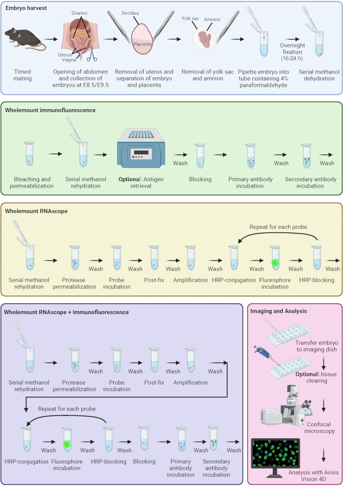
Figure 1: Immunofluorescence and RNAscope staining protocol. Schematic representing key stages of embryo harvest, immunofluorescence, RNAscope, combined immunofluorescence and RNAscope, sample imaging, and analysis. Colored boxes correspond to different protocol stages. Created in BioRender. Sparrow, D. (2026) https://BioRender.com/q6rmax8 Please click here to view a larger version of this figure.
結果
細胞周期のG2/M期にある遊走中の神経堤細胞の数を分析するため、本プロトコルに従ってE8.5胚を免疫蛍光染色しました。細胞周期のG2/M期を可視化するためにPHH3を標的とする抗体を、遊走中の神経堤細胞を可視化するためにSOX10を標的とする抗体を用いてサンプルを染色しました。さらに、適切な二次抗体で胚を染色しました。核はDAPIで染色しました。サンプルは、10倍対物レンズ(NA = 0.4)を装着したOlympus SpinSR回転ディスク共焦点顕微鏡を用いて撮影しました。画像は、Hamamatsu Orca Fusion BTカメラと50 µmピンホール回転ディスクを用いて取得しました。画像はタイル&ステッチ機能を用いてZスタックとしてキャプチャし、Z間隔は1.99 µmとしました。上皮間葉転換(EMT)による神経堤細胞の剥離とその後の遊走には、遊走前の神経堤細胞が細胞周期のS期またはG2/M期にあることが必要です20。ここでは、SOX10(マゼンタ)で示される遊走中の神経堤細胞集団の中で、PHH3染色(緑)で示される細胞周期のG2/M期の細胞を可視化することができました(Figure 2A)。対照群および処理曝露胚におけるG2/M期の遊走神経堤細胞数を定量化することで、本処理がG2/M期の遊走神経堤細胞数に影響を与えるか、したがって本処理がEMTによる神経堤の剥離を妨げる可能性があるかを判断できます。一部の胚では、解剖時に卵黄嚢が一部残存していました(Figure 2A’, 赤い矢印)。anti-PHH3抗体はマウスで作製されたため、本サンプルで多用されている抗マウス二次抗体による染色に対して、残存した卵黄嚢が感作されます。そのため、卵黄嚢全体が抗マウス抗体に結合した蛍光色素で強く蛍光を発します。この極端な例では、非特異的な染色がPHH3の定量化に影響を及ぼす可能性があるため、このサンプルは分析から除外すべきです。さらに、抗マウス抗体を使用すると、E8.5胚の心管に隣接して非特異的な「筋状の染まり(streak)」が生じます(Figure 2A’, 赤い矢印)。マウスで作製された一次抗体からの信号を定量化する際は、この領域を考慮する必要があります。
血管構造および心臓前駆細胞の分布を調べるため、本プロトコルを用いてE9.5胚を免疫蛍光染色しました。サンプルは、第二心臓領域を可視化するためのISLET1 (ISL1)、遊走する神経堤細胞を可視化するためのSOX10、静脈および毛細血管内皮細胞を可視化するためのENDOMUCIN (EMCN)を標的とする抗体、および適切な二次抗体を用いて染色しました。核はDAPIで染色しました。また、より深い深度のイメージングを行うために組織透明化法を用いました。サンプルは、10x対物レンズ (NA = 0.4) を装着したOlympus SpinSR回転円盤共焦点顕微鏡を用いて撮影しました。E9.5では、大動脈弓の一部を形成する心臓神経堤細胞の遊走 (SOX10、黄色) と、心房、流出路、および左心室の一部を形成する第二心臓領域前駆細胞 (ISL1、緑色) が観察されます21 (Figure 2B)。心臓前駆細胞の破綻は、先天性心疾患の主要な要因となります22,23。本手法を用いることで、心臓前駆細胞のパターニングと細胞数を可視化することが可能です。次の段階として、コントロール群と処置群の間で心臓前駆細胞のパターニングを比較し、介入が遊走を妨げるか、あるいは主要な細胞型の喪失を招くかを判定します。
神経堤細胞の段階とWntシグナリングの関係を明らかにするため、本プロトコルを用いてE8.5胚をRNAscopeで染色し、異なる遊走および分化段階にある神経堤細胞とWntシグナリングマーカーを検討した。神経堤細胞が出現する神経板境界(Msx1)、遊走神経堤細胞(Sox10)、および神経堤細胞の分化(Dlx2)を示すプローブを使用し、Wntシグナリングを示すプローブ(Sp5)と比較した。プローブの可視化には、TSA-vivid 520、570、650、およびOpal 780蛍光色素を用いた。サンプルは、Evident FV4000顕微鏡を使用し、10x対物レンズ(NA=0.4)、ピンホール径144 µm、ピクセルサイズ621 nmで撮像した。画像は、タイルおよびスティッチ機能を用いてZスタックとしてキャプチャし、Z間隔は4.32 µmとした。神経板境界(Msx1、緑)と遊走神経堤細胞(Sox10、マゼンタ)は頭部の異なる領域に位置しているが、細胞が神経管から遊走し始める部位で一部重複している(Figure 3A)。遊走神経堤細胞の一部の領域はDlx2(シアン)と共局在しており、一部の細胞が頭顔面分化へと進行していることが示唆された(Figure 3A)。Wntシグナリング(Sp5、黄)は神経板境界の領域に位置しており、これはWntシグナリングの調節が神経堤細胞の剥離と分化に必要であること24,25に関連しているが、同時に遊走神経堤細胞に隣接する独立した領域にも位置していた(Figure 3A)。
さらに、神経堤状態およびWntシグナリングのマーカーを染色することで、E9.5における神経堤細胞の遊走とWntシグナリングの関係を調べるための染色を行った。神経板境界を示すプローブ(Msx1)および遊走神経堤細胞(Sox10)が使用され、Wntシグナリングを示すプローブと比較された(Sp5)。プローブの可視化には、TSA-vivid 520、570、および650フルオロフォアを用いた。サンプルは、10倍対物レンズ(NA = 0.4)を装着したOlympus SpinSRスピニングディスク顕微鏡を用いて撮影した。ここで、神経板境界を確認できる(Msx1、緑色)、遊走中の神経堤細胞とは区別される(Sox10 マゼンタ)(図3B). Wntシグナリング(Sp5(黄色)は、体幹神経堤細胞が剥離している胚の背側領域、および頭部の特定の領域(1の周囲など)で強く認められます。st および 2nd 鰓弓、流出路の下方、および耳胞内(図3B本手法を用いて、対照群と処置群の間で神経堤細胞の空間的パターニングとWntシグナリングを比較することで、我々の介入が神経堤細胞の脱離および遊走を乱しているか、また、その乱れがWntシグナリングの変化に起因するかを判断することが可能になります。
神経板境界における細胞の細胞周期状態を決定するために、本プロトコルを用いて免疫蛍光染色とRNAscope染色の併用を行いました。神経板境界を示すRNAscopeプローブ(Msx1)を使用しました。細胞周期のG2/M期およびS期をそれぞれ可視化するため、PHH3およびPCNAを標的とする抗体を用いてサンプルを染色しました。その後、胚を適切な二次抗体でさらに染色し、核をDAPIで染色しました。サンプルの撮像には、10倍対物レンズ(NA = 0.4)を装着したOlympus SpinSRスピニングディスク顕微鏡(Figure 4A,B)、または10倍対物レンズ(NA = 0.4)、127 µmピンホール、ピクセルサイズ311 nmに設定したEvident FV4000共焦点顕微鏡(Figure 4B’)を使用しました。ここで、G2/M期(PHH3、黄色)とS期(PCNA、マゼンタ)の両方の細胞が神経板境界と重複していることが確認できます(Figure 4A)。この方法を用いることで、神経板境界内における各細胞周期段階の細胞の割合を定量化し、これらの割合が処理群によって変化するかどうかを判断できます。この胚において顕著なのは、微細ピンセットによる過度な操作で胚に解剖上の損傷が生じたことによる穴です。このことは、特に胚が非常に脆弱なE8.5において、損傷を防ぐために解剖時に細心の注意を払う必要があることを強調しています。
RNAscopeと免疫蛍光染色を組み合わせると、RNAscope単独で実施した場合よりもRNAscopeプローブの染色強度が低下することがあります。近接した蛍光色素(例:FluoresceinとCy3)を用いて、非常に明るく蛍光する一次抗体と組み合わせた場合、明るいチャンネルから暗いチャンネルへの信号のブリードスルーが生じる可能性があります(図4B)。これを防ぐには、非常に明るい抗体の濃度をより希釈して使用するか、スペクトル的に乖離した蛍光色素を選択するか、あるいはサンプルのイメージングパラメータを変更することが有効です。回転円盤共焦点顕微鏡は胚のイメージング速度が非常に速いですが、固定された透過窓を持つバンドパス放出フィルターを使用しているため、特定の蛍光色素に合わせて検出窓を動的に狭めることはできません。一方、Evident FV4000などのポイントスキャニング顕微鏡を使用すると、オペレーターがナノメートル単位の精度で検出窓を狭めることができるため、放出スペクトルがわずかに重複する蛍光色素を使用した場合でもブリードスルーを低減させることが可能です(図4B’)。
E8.5胚において、細胞周期の各段階にある細胞の割合を決定するため、本プロトコルを用いて、細胞周期のS期およびG2/M期における核の割合と信号強度を解析した。細胞周期のG2/M期およびS期をそれぞれ可視化するため、PHH3およびPCNAを標的とする抗体を用いてサンプルを染色した。さらに、適切な二次抗体を用いて胚を染色した。核はDAPIで染色した。サンプルの撮像には、10倍対物レンズ(NA = 0.4)を装着したOlympus SpinSRスピニングディスク顕微鏡を使用した。すべての核、PHH3陽性核、PCNA陽性核、および二重陽性核の特定には、Zeiss Arivis Proを使用した(図5A)。この手法を用いることで、G2/M期の細胞の割合(PHH3+) および S (PCNA+細胞周期の各相(図5B)、および個々の核におけるPHH3またはPCNA染色の強度(図5C)。PCNAの割合がわずかに高かったことがわかります。+ 頭部および胚全体と比較した心臓領域の核(図5B)。さらに、頭部ではPHH3の割合が高かった。+ および、心臓および胚全体と比較した二重染色された核(図5B)。領域間において、PHH3またはPCNAの強度の明らかな差は認められなかった(図5C). これらのデータは単一の代表的な胚(n = 1)から得られたものであり、解析ワークフローを示すために提示しています。推測統計解析は行っていません。以上の手法により、心臓および頭蓋顔面の発達に不可欠な発達段階における細胞周期伝播のパターンを決定することが可能になります。また本手法を用いることで、我々の処置が胚の異なる領域における細胞周期伝播に影響を与えるかどうかを判断できるようになります。
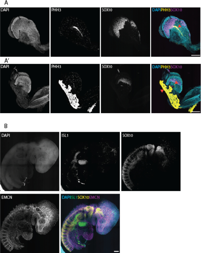
図2E8.5およびE9.5胚におけるタンパク質の免疫蛍光染色。 (A, A’E8.5マウス胚を用い、細胞周期のG2/M期にある細胞を可視化するためのPHH3、遊走中の神経堤細胞を可視化するためのSOX10、および核を可視化するためのDAPIによる免疫蛍光染色を行った。N = 1回の実験から得られた11個の胚。BE9.5胚において、第二心野前駆細胞を可視化するためのISL1、遊走中の神経堤細胞を可視化するためのSOX10、毛細血管および静脈を可視化するためのEMCN、および核を可視化するためのDAPIで染色を行った。赤色の矢頭は卵黄嚢の非特異的な染色を示し、 抗マウス二次抗体による胚内部の非特異的染色(n = 1回のエクスペリメントから得られた15個の胚)。スケールバー = 200 µmDAPI: 4′,6-ジアミジノ-2-フェニルインドール; PHH3: リン酸化ヒストンH3; EMCN: エンドムシン この図の拡大版を表示するには、ここをクリックしてください。
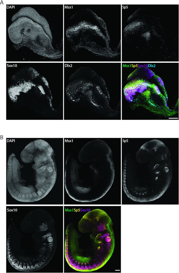
図3RNAscopeによるE8.5およびE9.5胚の転写物の染色。 (A) E8.5胚をRNAscopeにより染色し、以下の標的プローブを用いた。 Msx1 神経板境界を可視化するために、 Sox10 遊走する神経堤を可視化するために、 Dlx2 分化中の神経堤を可視化し、 Sp5 Wntシグナリングについて。1回の実験から得られたn = 13個の胚。(BE9.5胚を、以下の標的プローブを用いてRNAscopeで染色した。 Msx1 神経板境界を可視化するために、 Sox10 遊走する神経堤を可視化し、 Sp5 Wntシグナリングを可視化するため。n = 1回の実験から得られた4個の胚。スケールバー = 200 µm. この図の拡大版を表示するには、ここをクリックしてください。
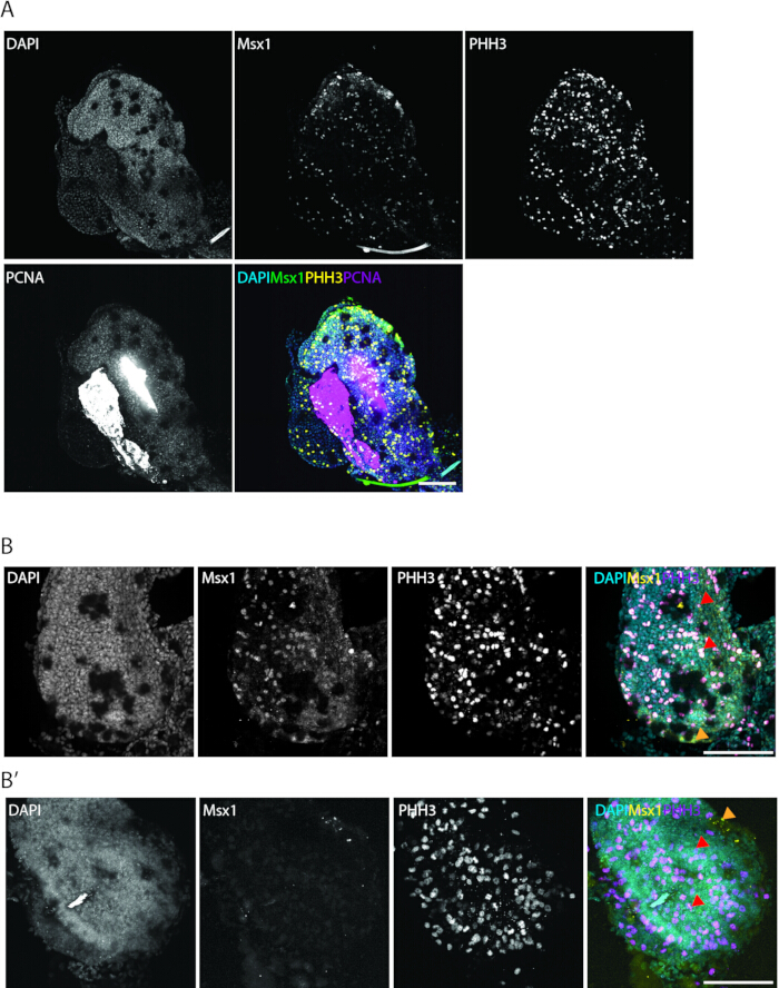
図 4: E8.5胚における免疫蛍光染色とRNAscopeの併用。(A, B, B’) E8.5胚において、神経板境界を可視化するためにMsx1を標的とするプローブを用いてRNAscopeを行い、さらにS期の細胞を可視化するためにPCNAの免疫蛍光染色を、細胞周期のG2/M期の細胞を可視化するためにPHH3抗体を用いた免疫蛍光染色を行った。オレンジ色の矢頭は特異的なMsx1 染色を、赤色の矢頭はブリードスルーによる蛍光 (B)、またはMsx1チャンネルへのブリードスルーを伴わない特異的なPHH3染色 (B') を示す。N = 1回の実験における胚2個。スケールバー = 200 µm。この図の拡大版を表示するには、ここをクリックしてください。
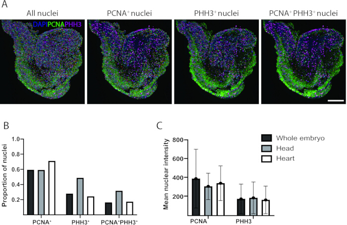
図 5: Arivis Proを用いたE8.5胚における細胞周期ステージの解析。(A) E8.5マウス胚を、細胞周期のS期の細胞を可視化するためのPCNA(緑)、G2/M期の細胞を可視化するためのPHH3(マゼンタ)、および核を可視化するためのDAPI(青)で免疫蛍光染色した。検出された3Dオブジェクト(多色の球体)を重ね合わせ、Zeiss Arivis Proの4Dビューアを用いて可視化した。(B) グラフは、単一胚の全身、頭部、および心臓におけるPCNA+、PHH3+、および二重陽性核の割合を示している。(C) グラフは、単一胚の全身、頭部、および心臓における核1個あたりのPCNAおよびPHH3染色の平均強度を示している。円は平均値を表し、エラーバーは単一サンプル内のすべての核の標準偏差を表す。グラフはGraphPad Prismを用いて作成した。スケールバー = 200 µm。定量解析はn = 1胚に対して実施した。推測統計は行われていない。エラーバーは個々の核間の標準偏差を示す。 3D: 三次元; DAPI: 4′,6-diamidino-2-phenylindole. この図の拡大版を表示するには、ここをクリックしてください。
ディスカッション
本稿では、E8.5およびE9.5のホールマウント胚における遺伝子およびタンパク質発現を空間的に解析するための最適化された手法について説明します。これらの手法は、従来のRNA in situ ハイブリダイゼーションや切片の免疫蛍光染色と比較して、空間分解能とマルチプレックス能力が向上しています。本プロトコールは、マウス胚における発生経路を調べるための最近の既存プロトコールに基づいています。最近のあるプロトコールでは、RNAscopeと免疫蛍光染色を用いて胚内のWntシグナルを解析していますが、ホールマウント胚ではなく切片を染色しています26。また、別の最近の研究では、E8.5~E10.5のホールマウントマウス胚を用いてホールマウントRNAscopeおよび免疫蛍光染色を行っていますが27、著者らはこれら2つの染色技術を組み合わせておらず、C4プローブとOpal 780蛍光色素を用いた4番目のRNAscopeチャネルの染色も行っていませんでした。免疫蛍光染色とRNAscopeの組み合わせは、以前にホールマウントE3.5胚で報告されており、そこでは免疫蛍光プロトコールの完了後にRNAscopeが実施されています28。我々は、より後期の胚でこの正確なプロトコールを試行したわけではありませんが、E8.5胚において、免疫蛍光プロトコールの一次抗体と二次抗体のインキュベーションの間にRNAscope染色を挟み込んだ場合、抗体染色の結果が悪くなることが分かりました。これは、大きな胚でRNAscopeを行う際にプロテアーゼ処理が必要となるためと考えられ、E3.5マウス胚を用いた研究ではこの処理は不要でした。プロテアーゼ処理は結合した抗体の完全性に影響を及ぼす可能性があるため、この系においてRNAscopeと免疫蛍光染色の順序を入れ替えても成功する可能性は低いと考えられます。筋線維における別の最近の研究では、免疫蛍光染色の前にRNAscopeを行うことで、これら2つのプロトコールを組み合わせています29。本プロトコールと同様に、その研究でも免疫蛍光染色の前にRNAscopeを実施していますが、ホールマウントマウス胚での検証は行われておらず、またC4プローブとOpal 780蛍光色素を用いて追加のRNAscopeチャネルを組み込んだRNAscopeも実施されていませんでした。
マルチプレックス法を用いた胚のホールマウント染色の能力は、主要な転写産物やタンパク質のマッピング、あるいは異なる段階の胚における前駆細胞種や発生シグナル伝達経路の標識を可能にし、発生生物学において広範な応用が期待されます。我々はこれらの技術を用いて、心前駆細胞の分布(図 2B)、遊走および分化の異なる段階にある神経堤細胞(図 3)、Wntシグナリング(図 3)、および細胞周期の段階(図 2, 図 4, 図 5)をマッピングすることができました。使用するプローブや抗体を変更することで、この段階の胚に存在する限り、任意の細胞種やシグナル分子をこれらの技術で解析することが可能です。本プロトコルではE8.5およびE9.5に焦点を当てていますが、組織の透過処理、インキュベーション時間、および組織透明化を最適化することで、より若い、あるいはより高齢の胚を染色できる可能性があります。
しかし、全胚(whole-mount)におけるタンパク質および転写産物の発現をマルチプレックス解析できる能力が向上したことで、さらなる課題が生じています。第一に、全胚サンプルの解析は、切片を用いた免疫蛍光染色やRNAscopeに比べて時間がかかります。切片を用いた解析は通常1〜2日で完了しますが、全胚の場合は数日を要します。さらに、全胚サンプルを使用する場合、十分なサンプル深さと解像度を確保するために、顕微鏡のパラメータを慎重に検討する必要があります。そのため、最大で〜までイメージング可能な顕微鏡が必要です。 700 µm 組織が厚いため、より大きな胚では組織透明化法を用いる必要があります。さもなければ、試料深部の構造を見逃す可能性があります。加えて、試料の厚みにより、ワイドフィールド顕微鏡で結像させると焦点面外からの光が大量に導入されます。共焦点顕微鏡は焦点面外からの信号を除去できるため、面外信号を排除しながら試料内部を撮像することが可能であり、こちらが推奨されます。さらに、スピニングディスク共焦点顕微鏡は多くの場合、画像取得時間を短縮できますが、ポイントスキャン共焦点顕微鏡に比べると蛍光検出の精密な制御に劣ります。また、胚のサイズも課題となります。多くの顕微鏡では、タイルスキャンを行わずに胚を撮像できるほどの十分な視野が確保されていないためです。これにより、画像内にステッチングアーチファクト(例: 図 2B)。サンプルのマルチプレックス化は、チャンネル間のブリードスルー(例: 図4B), これは、検出ウィンドウを狭めることができるポイント走査型共焦点顕微鏡を選択することで軽減でき、蛍光色素の放出スペクトルにわずかな重複がある場合に有効です。Opal 780蛍光色素を使用すると、単一のサンプル内でさらに多くの標的をマルチプレックスすることが可能です。この系を検出するには、近赤外線でのイメージングが可能な顕微鏡が必要となります。この機能は、大半の光学顕微鏡では利用できません。
イメージングのためのサンプルの固定についても、慎重に検討する必要があります。マルチウェルチャンバースライドでイメージングを行う際など、サンプルを遊泳させた状態にすると、サンプルが常に正確に同じ角度で固定されるとは限りません。これにより、胚のどの部分がカメラや検出器に近いかによって染色の強度に差が生じ、その後の強度解析を行う際に困難が生じることがあります。さらに、マルチウェルチャンバースライドを使用する場合、ウェルの端がイメージング範囲に入り込み、画像にアーティファクトが生じることがあります。キャビティスライドのように胚を固定する方法は、方向性を維持するのに役立ちますが、胚を損傷させたり圧縮したりしやすく、構造の体積解析を困難にする可能性があります。
本プロトコルに従う際は、いくつかの検討事項があります。免疫蛍光染色において、抗原賦活化の際に胚を解離させないよう注意が必要です。特に若齢の胚を解析する場合は注意してください。これを避けるために、Tris/EDTAなどの代替バッファーの使用や、タンパク質分解による賦活化法など、他の抗原賦活化法を用いることが有効な場合があります。また、胚のサイズが小さい、あるいは大きい場合には、抗体インキュベーション時間の最適化が有用な可能性があります。一次抗体の選択には慎重な検討が必要です。多くの抗体がマウスで作成されていますが、抗マウス抗体を使用すると、残留した卵黄嚢に結合して強い蛍光を発することがあります。これは、AlexaFluor 488 (Figure 2) および AlexaFluor 647 (Figure 4) が結合した抗マウス二次抗体を用いた場合に確認できます。当研究室では他の蛍光色素はテストしていませんが、蛍光強度が異なる可能性があるため、さらなる最適化が必要になる場合があります。この現象は、抗ウサギ抗体 (Figure 2, Figure 4, Figure 5) または抗ラット抗体 (Figure 2B) を使用したチャンネルでは見られません。したがって、可能な限り他種で作成された一次抗体を使用することを推奨します。
RNAscopeにおいては、プロテアーゼ処理の時間を最適化することが極めて重要です。処理時間が短すぎるとプローブの浸透が不十分になり、長すぎると試料が完全に剥離してしまう可能性があるためです。プロテアーゼ処理時間を最適化する際は、時間を1分ずつ調整することを推奨します。また、プローブや抗体が適切に機能したかを確認するために、適切なコントロールを用いることが最善の方法です。陰性コントロールとしては、同ステージの胚を同時に染色し、プローブまたは一次抗体を添加しない個体を使用するか、あるいは免疫蛍光染色ではIgGアイソタイプコントロールを、RNAscopeでは陰性コントロールプローブを用いて、観察された染色が本物であることを確認します。また、目的の遺伝子や転写産物を発現していることが分かっている同サイズの組織を陽性コントロールとして用いることも、染色の成功を確認する上で有用です。
全体として、本プロトコルはE8.5およびE9.5のマウス胚全 mountにおけるタンパク質および転写産物の発現を可視化するための堅牢で最適化された手法であり、正常な胚発生および疾患における細胞・分子メカニズムを研究する上で大きな可能性を秘めています。
開示事項
著者は、競合する利害関係がないことを宣言します。
謝辞
著者らは、本原稿に含まれる顕微鏡観察および画像解析における技術的支援を提供してくださった、オックスフォード大学人類遺伝学センターのCellular Imaging Core facilityのチームに感謝いたします。また、胚を生成するための動物の飼育および計画交配を支援してくださった、オックスフォード大学Biomedical Servicesのスタッフに感謝いたします。
本研究の資金提供は、British Heart Foundation Senior Fellowship FS/SBSRF/22/31022 (DBS)、Additional Ventures Single Ventricle Fund (DBS)、John Fell Fund、University of Oxford 0016065 (VSR)、およびMedical Sciences Internal Fund, University of Oxford 0016707 (VSR) によるものである。
材料
| 名前 | 会社 | カタログ番号 | コメント |
|---|---|---|---|
| プラスチック器具/ガラス器具 | |||
| 3ml パスツールピペット 低密度ポリエチレン (LDPE) 目盛り付き | Wheaton | 711116 | |
| Eppendorf Safe-lockチューブ 1.5ml マイクロチューブ | Eppendorf | 0030 120.086 | |
| Ibidi µ18ウェルスライド | Ibidi | 81817 | #1.5H ガラスカバースリップ、未処理 |
| Menzel X1000 カバーガラス 22x50 mm #1.5 (0.16-0.19mm) | Thermo Scientific | 17284904 | |
| 凹み付き顕微鏡スライドガラス | Marienfeld Superior | 1320000 | |
| セーフシールマイクロチューブ 2ml | Sarstedt | 72.695.500 | 2ml Eppendorfチューブ、ラウンドボトム |
| 溶液/緩衝液 | |||
| 1x 抗体希釈液/ブロッキング液 | Akoya Biosciences | ARD1001EA | |
| Ambion™ RnaseZap™ RNase除染溶液 | Ambion | 9780.9782 | |
| クエン酸アンマスキング緩衝液 | Vector Labs | H-3300 | 抗原賦活化溶液と表記された、 クエン酸ベースの |
| ジメチルスルホキシド (DMSO) | Merck (Sigma-Aldrich) | D8418 | |
| ハンクス平衡塩溶液 10倍濃縮液 | Merck (Sigma-Aldrich) | H4641 | |
| 過酸化水素溶液 | Merck (Sigma-Aldrich) | H1009 | 30% (w/w) H2O溶液 |
| メタノール | Merck (Sigma-Aldrich) | 32213-2.5L-M | |
| 正常ロバ血清 | Abcam | Ab7475 | 100%ストック濃度、 最終濃度10% |
| パラホルムアルデヒド(PFA)粉末 | Merck (Sigma-Aldrich) | 158127-500g | 水で4%に希釈する。ドラフトチャンバー内で調製すること。加熱ブロック上で攪拌し、溶解を促進させるために少量のNaOHを加える。pH 7.2-7.6 |
| リン酸緩衝生理食塩水 (PBS) | Merck (Sigma-Aldrich) | P4417 | 蒸留水200mlにつきタブレット1錠 |
| Multiplex Fluorescent Reagent Kit v2用RNAscope 4-Plex Ancillary Kit | ACD (Bio-Techne) | 323120 | HRP-C4およびHRPブロッカーを含む |
| RNAscope™ マルチプレックス蛍光検出キット v2 | ACD (Bio-Techne) | 323110 | Protease PlusおよびProtease IIIを含む プロテアーゼIV、過酸化水素、TSA緩衝液、 Amp1/2/3、Hrp-C1/2/3、HRPブロッカーおよびDAPI |
| 20倍濃度塩化ナトリウム-クエン酸ナトリウム(SSC)緩衝液 | Fisher Bioreagents | BP-1325-1 | 蒸留水を用いて0.2倍に希釈する。 |
| 組織透明化試薬 Cubic-R+(M)[動物用] | 東京化成工業 | T3741 | |
| トリトン™ 100倍 | Merck (Sigma-Aldrich) | X100 | |
| Tween® 20 | Merck (Sigma-Aldrich) | P7949 | |
| 超純水™ 0.5M EDTA (pH 8) | Invitrogen | 15575020 | |
| 一次抗体 | |||
| エンドムシン抗体(V.7C7) | サンタクルーズ | SC-65495 | 1:50に希釈して使用してください。 |
| Islet 1およびIslet 2抗体 | Developmental Studies ハイブリドーマバンク | 34.4DS-5 | グリセロールを用いて50%に希釈する。1:50の希釈率で使用する。 |
| PCNA (PC10) マウスモノクローナル抗体 | 細胞シグナル伝達技術 | 2586S | 1:500希釈で使用してください。 |
| P-histone H3 (Ser10) (6G3) マウスモノクローナル抗体 | 細胞シグナル伝達技術 | 9706S | 1:500の希釈倍率で使用する |
| P-histone H3 (Ser10) (D7N8E) XP® ウサギモノクローナル抗体 | セルシグナリングテクノロジー | 53348S | 1:500に希釈して使用する |
| Sox10 (E6B6I) XP® ウサギモノクローナル抗体 | 細胞シグナル伝達技術 | 69661S | 1:500に希釈して使用する |
| 二次抗体/核染色剤 | |||
| AlexaFluor® 488標識Affinipure® ドンキー抗マウスIgG (H+L) | Jackson Immunoresearch | 715-545-151 | 1:500希釈で使用する |
| AlexaFluor® 647標識Affinipure® ドンキー抗ラットIgG (H+L) | Jackson Immunoresearch | 712-605-153 | 1:500に希釈して使用してください。 |
| AlexaFluor® 647標識Affinipure® ドンキー抗マウスIgG (H+L) F(ab')2フラグメント | Jackson Immunoresearch | 715-606-150 | 1:500の希釈率で使用してください。 |
| Cy™3 Affinipure® ドンキー抗ウサギIgG (H+L) | Jackson Immunoresearch | 711-165-152 | 1:500に希釈して使用する |
| DAPI | Merck (Sigma-Aldrich) | D9542 | 使用量 1 µg/ml |
| RNAscopeプローブ | |||
| RNAscope® プローブ - Mm Sp5-C4 | ACD (Bio-Techne) | 405681-C4 | C4プローブ |
| RNAscope® プローブ - Mm-Dlx2-C3 | ACD (Bio-Techne) | 555951-C3 | C3プローブ |
| RNAscope® プローブ - Mm-Msx1 | ACD (Bio-Techne) | 421841 | C1プローブ |
| RNAscope® プローブ - Mm-Sox10-C2 | ACD (Bio-Techne) | 435931-C2 | C2プローブ |
| RNAscope蛍光色素 | |||
| Opal 780試薬パック | Akoya Biosciences | FP1501001KT | Opal 780試薬およびOpal TSA-DIGを含む。 ジメチルスルホキシド |
| TSA-vivid™ フルオロフォア 520 | ACD (Bio-Techne) | 323271 | 現在はClariTSAです。™ フルオロフォア 520 |
| TSA-vivid™ フルオロフォア 570 | ACD (Bio-Techne) | 323272 | now ClariTSA™ フルオロフォア 570 |
| TSA-vivid™ フルオロフォア650 | ACD (Bio-Techne) | 323273 | now ClariTSA™ フルオロフォア650 |
| 装置/ソフトウェア | |||
| Fluoview FV4000レーザースキャニング 顕微鏡 | 明白な | FV4000 | 励起レーザー:405/488/561/640/730 nm。 検出波長(図3):430-470、500-540、570-620、 650-710、750-850 nm。検出波長(図4)430-470、 500-531, 570-620 nm. |
| GraphPad Prism 10 | GraphPad | v10.6.1 | |
| 加熱ブロック | 助成金 | QBT1 | |
| Hybrigene ハイブリダイゼーションオーブン | Techne (Bibby Scientific) | FHB4DD | |
| Ixplore IX83 SpinSR 超解像顕微鏡システム | Olympus | ixplore-ix83-spinsr | 励起レーザー:405/488/561/640 nm。 エミッションフィルター:447/60、525/50、617/73、685/40。 |
| Zeiss Arivis Pro | Carl Zeiss Microscopy GmbH | v. 4.5(旧 Arivis Vision 4D) | |
| Zeiss Arivis SISコンバーター | Carl Zeiss Microscopy GmbH | v. 4.3.0 |
参考文献
- Bruter AV, Varlamova EA, Okulova YD, Tatarskiy VV, Silaeva YY, Filatov MA. Genetically modified mice as a tool for the study of human diseases. Mol Biol Rep. 2024;51(1):135.
- Rashbrook VS, Brash JT, Ruhrberg C. Cre toxicity in mouse models of cardiovascular physiology and disease. Nat Cardiovasc Res. 2022;1:806–16.
- Breschi A, Gingeras TR, Guigo R. Comparative transcriptomics in human and mouse. Nat Rev Genet. 2017;18(7):425–40.
- Mole MA, Weberling A, Zernicka-Goetz M. Comparative analysis of human and mouse development: From zygote to pre-gastrulation. Curr Top Dev Biol. 2020;136:113–38.
- Krishnan A, Samtani R, Dhanantwari P, Lee E, Yamada S, Shiota K, et al. A detailed comparison of mouse and human cardiac development. Pediatr Res. 2014;76(6):500–7.
- Anderson RH, Bamforth SD. Morphogenesis of the Mammalian Aortic Arch Arteries. Front Cell Dev Biol. 2022;10:892900.
- Wessels A, Sedmera D. Developmental anatomy of the heart: a tale of mice and man. Physiol Genomics. 2003;15(3):165–76.
- Gall JG, Pardue ML. Formation and detection of RNA-DNA hybrid molecules in cytological preparations. Proc Natl Acad Sci U S A. 1969;63(2):378–83.
- John HA, Birnstiel ML, Jones KW. RNA-DNA hybrids at the cytological level. Nature. 1969;223(5206):582–7.
- Buongiorno-Nardelli M, Amaldi F. Autoradiographic detection of molecular hybrids between RNA and DNA in tissue sections. Nature. 1970;225(5236):946–8.
- Dakou E, Vanbekbergen N, Corradi S, Kemp CR, Willems E, Leyns L. Whole-mount in situ hybridization (WISH) optimized for gene expression analysis in mouse embryos and embryoid bodies. Methods Mol Biol. 2014;1211:27–40.
- Anderson R. Multiplex fluorescence in situ hybridization (M-FISH). Methods Mol Biol. 2010;659:83–97.
- Kearney L. Multiplex-FISH (M-FISH): technique, developments and applications. Cytogenet Genome Res. 2006;114(3-4):189–98.
- Burnett R, Guichard Y, Barale E. Immunohistochemistry for light microscopy in safety evaluation of therapeutic agents: an overview. Toxicology. 1997;119(1):83–93.
- Coons AH, Creech HJ, Jones RN. Immunological properties of an antibody containing a fluorescent group. P Soc Exp Biol Med. 1941;47(2):200–2.
- Bardot E, Tzavaras N, Benson DL, Dubois NC. Quantitative Whole-mount Immunofluorescence Analysis of Cardiac Progenitor Populations in Mouse Embryos. J Vis Exp. 2017(128).
- Wang F, Flanagan J, Su N, Wang LC, Bui S, Nielson A, et al. RNAscope: a novel in situ RNA analysis platform for formalin-fixed, paraffin-embedded tissues. J Mol Diagn. 2012;14(1):22–9.
- Erben L, Buonanno A. Detection and Quantification of Multiple RNA Sequences Using Emerging Ultrasensitive Fluorescent In Situ Hybridization Techniques. Curr Protoc Neurosci. 2019;87(1):e63.
- De Bono C, Lescroart F, Zaffran S. How to Study Gene Expression and Gain of Function of Hoxb1 in Mouse Heart Development. Methods Mol Biol. 2025;2889:121–37.
- Zhao R, Moore EL, Gogol MM, Unruh JR, Yu Z, Scott AR, et al. Identification and characterization of intermediate states in mammalian neural crest cell epithelial to mesenchymal transition and delamination. Elife. 2024;13.
- Guijarro C, Kelly RG. On the involvement of the second heart field in congenital heart defects. C R Biol. 2024;347:9–18.
- Bradshaw L, Chaudhry B, Hildreth V, Webb S, Henderson DJ. Dual role for neural crest cells during outflow tract septation in the neural crest-deficient mutant Splotch(2H). J Anat. 2009;214(2):245–57.
- Zawada D, Kornherr J, Meier AB, Santamaria G, Dorn T, Nowak-Imialek M, et al. Retinoic acid signaling modulation guides in vitro specification of human heart field-specific progenitor pools. Nat Commun. 2023;14(1):1722.
- Rabadan MA, Herrera A, Fanlo L, Usieto S, Carmona-Fontaine C, Barriga EH, et al. Delamination of neural crest cells requires transient and reversible Wnt inhibition mediated by Dact1/2. Development. 2016;143(12):2194–205.
- Bhattacharya D, Rothstein M, Azambuja AP, Simoes-Costa M. Control of neural crest multipotency by Wnt signaling and the Lin28/let-7 axis. Elife. 2018;7.
- Kishimoto K, Furukawa KT, Luz-Madrigal A, Yamaoka A, Matsuoka C, Habu M, et al. Bidirectional Wnt signaling between endoderm and mesoderm confers tracheal identity in mouse and human cells. Nat Commun. 2020;11(1):4159.
- De Bono C, Liu Y, Ferrena A, Valentine A, Zheng D, Morrow BE. Single-cell transcriptomics uncovers a non-autonomous Tbx1-dependent genetic program controlling cardiac neural crest cell development. Nat Commun. 2023;14(1):1551.
- Hazra R, Spector DL. Simultaneous visualization of RNA transcripts and proteins in whole-mount mouse preimplantation embryos using single-molecule fluorescence in situ hybridization and immunofluorescence microscopy. Front Cell Dev Biol. 2022;10:986261.
- Kann AP, Krauss RS. Multiplexed RNAscope and immunofluorescence on whole-mount skeletal myofibers and their associated stem cells. Development. 2019;146(20).
再版と許可
この記事は公開されました
動画は近日公開