本研究では、中国南部の3つの客家文化生態保護区を対象に、生態系と遺産を組み合わせた二層のネットワークを構築しました。パーコレーション解析により、生態系レイヤーとマッピングされた遺産目録レイヤーのそれぞれについて異なる構造的堅牢性の閾値を特定し、さらに復元優先度指数を用いて影響力の強いパッチを特定しました。このフレームワークは、各保護区における復元およびモニタリングの選択肢について、エビデンスに基づく比較を可能にします。
この記事について
サマリー
要約
本研究は、生態学的コネクティビティと無形文化遺産を結合された2層グラフとしてモデル化する、二層生態・遺産ネットワーク(DEHN)フレームワークを提案し、中国南部の3つの客家文化生態保護区(74,547 km2)に適用した。具体的には、土地被覆データ(2000–2023年)にMSPA-liteを用いることで、233ノード、799エッジの生態ネットワークを構築し、10 kmの距離減衰スキームを介して23ノード、73エッジの遺産ネットワークと結合させた。さらに、パーコレーション攻撃により、生態層の閾値0.690および遺産層の閾値0.925という臨界値が明らかになり、生態ネットワークは無形文化遺産(ICH)目録ネットワークよりも早く連結性を失うことが示された。復元優先度指数(Restoration Priority Index)により、ティア1(最上位)の47パッチと高優先度の46パッチが特定され、梅州市に上位層の75%が集中していることが分かった。反実仮想シミュレーションでは、エッジコストの削減が崩壊閾値を変化させる一方で、パッチの喪失は閾値を98.4%低下させることが示され、新たなステッピングストーンパッチによるトポロジー的拡張が必要であることが判明した。DEHNフレームワーク全体として、密度正規化された比較(23.3対3.21)を行い、生態層は単位コネクティビティあたりの回復力がより高いことを示しており、文化生態保護区における結合的な復元計画に転用可能なテンプレートを提供する。DEHNフレームワークは、持続可能な開発目標(SDG)11.4(「世界の文化遺産および自然遺産の保護・保存のための努力を強化する」)および愛知目標11(陸域の少なくとも17%を保全する)に関連している。特定されたパーコレーション閾値(生態層 f_C = 0.690、遺産層 f_C = 0.925)は、文化生態保護区(CEPZ)の管理がネットワークの回復力を崩壊閾値以上に維持しているかを評価するための定量的なベンチマークとなる。連鎖的崩壊を引き起こすティア1(最上位)を構成する47パッチ(生態ネットワークの20%)という知見は、これらのトポロジー的に重要なパッチを優先していない現在のCEPZ境界指定が、SDG 11.4の目標達成には不十分である可能性を示唆している。著者らは、CEPZ管理計画にネットワーク回復力閾値をモニタリング指標として組み込み、合意された f_C が0.50(ネットワーク崩壊の操作的定義)を上回っているかを毎年報告することを推奨している。
概要
世界的に、生態学的・文化的景観が結合した地域は、都市化、農村部の人口減少、および気候変動によって同時に再編されており、生物物理学的な健全性と遺産の継続性の双方が脅かされています1,2。特に山岳文化景観は脆弱であり、人口密度の高い多くの地域の最後の連続的な森林コアを保持しながら、不釣り合いなほど多くの無形文化遺産が集中しています3。持続可能な開発目標(SDG)11.4および愛知目標11は、世界の文化・自然遺産の保護と、生態学的に代表的な生息地の保護を共同で求めていますが、10年間のモニタリングによれば、多くの管轄区域においてこれら2つの目標が非同期に展開していることが示されています4。中国では、国家的な文化生態保護区(CEPZ)プログラムにより、生態学的な健全性と無形遺産を一つのシステムとして保全すべき一貫した領域単位が指定されています5。しかし、制度開始から15年以上が経過した現在でも、CEPZ政策は、2つのレイヤーを接続する空間的メカニズムではなく、ほぼ排他的にインベントリベースの指標を通じて評価されてきました。そのため、CEPZ内の生態学的サブシステムと遺産サブシステムが、異なるストレス要因に反応して同期的に劣化するのか、あるいは異なる軌跡をたどるのかについては、いかなるスケールにおいても経験的に解明されていません。
生息地マトリックスの分布と透過性を再編成することにより、景観分断化はエコシステムサービスの提供を支えるコネクティビティそのものを変化させます6。分断化は通常、パッチ密度、形状の不規則性、土地被覆のシャノン多様性などの景観パターン指標によって定量化され、しばしばムービングウィンドウ解析と組み合わせて行われます7。より最近では、形態学的空間パターン解析(MSPA)および本研究で採用したその軽量版(MSPA-lite)が、中国の地域生態学におけるコア・エッジ・ブリッジの生息地構造を分離するための主要な手法として登場しました8,9。これらの形態学的ツールは有用ですが、生物やエコシステムサービス(ES)の流れに関しては根本的に非空間的です。つまり、生息地断片の分布を記述してはいても、どのような経路で生態学的サービスが生息地コア間に伝播するかについては言及していません10。この制約は、生態学的および遺産的な実体が景観全体で機能的に接続されているという政策的前提を持つ中国のCEPZにおいて特に深刻です。しかし、メカニズムを明示した空間モデルがなければ、景観指標だけでは、CEPZ管理が保護すべきコネクティビティ経路を明らかにすることはできません。
グラフ理論および回路理論に基づくコネクティビティモデルは、生態系サービスにおけるこの空白を部分的に埋めてきた。土地利用マップから導出された抵抗面的における最小コスト経路(LCP)解析は、現在では生息地コア間の生態学的コリドーを画定するための標準的なツールとなっている11,12。回路理論(Circuitscape)は、景観を抵抗ネットワークとして扱い、多経路のフロー確率を算出する13。近年のマルチプレックスネットワークによる統合研究では、これらの単一層ツールを拡張して、生態系サービスの供給・需要フローを表現できることが示されている14,15。文化遺産側については、空間的な定量化が異なる方向で進展してきた。カーネル密度推定(KDE)は、無形文化遺産のクラスター表現のデフォルトとなっており16、組み合わせグラフ(通常は申告された遺産地点上のドロネー三角形分割またはk近傍ネットワーク)が、遺産資産の離散的な関係構造を捉えている17。しかし、生態学的ネットワークと遺産ネットワークは、ほぼ常に並行した単一層オブジェクトとして扱われてきた18,19。両方の層によって共同で制御される伝播ダイナミクスを持つ、それらが結合したsupra-network(超ネットワーク)となる可能性は、CEPZスケールではまだ実用化されていない20,21。その結果、漸進的なストレッサーの除去に伴い、結合された二層ネットワークがその巨大連結成分を喪失するレジリエンスしきい値は、依然として不明なままである。
ノードが参加者を表し、エッジが相互作用をコード化するネットワークモデルは、このギャップを埋めるための数学的装置を提供します22。マルチレイヤーおよびマルチプレックスネットワークは、同じアクターが構造的に異なる相互作用レジームに参加するシステムへとグラフ表現を一般化し23、レイヤー間の結合、レイヤーをまたいだ参加、およびレイヤー固有のレジリエンスを測定するための簡潔なメカニズムを提供します。生態学的ネットワーク研究では、パーコレーションに基づくノード除去シミュレーションを用いて、最大連結成分が崩壊する臨界分率 f* を特定することが、構造的レジリエンスの広く受け入れられているプロキシとして用いられてきました24。これらのツールを結合された生態系・遺産アーキテクチャに拡張するには、(i) 生息地のコアと遺産地点の間の空間的近接性を反映した明示的なレイヤー間結合スキーム、(ii) 各レイヤーに独立して標的を絞り、レイヤー固有の脆弱性を分離する攻撃プロトコル、および (iii) 結合ネットワークの診断結果を実効性のある復元目標へと変換する複合優先度指標が必要となります。本分析で開発した二層生態系・遺産ネットワーク(Dual-layer Ecological–Heritage Network: DEHN)フレームワークは、これら3つの要件を具体化し、それに基づき、マルチCEPZスケールにおける両レイヤーのレジリエンス閾値と、それらのレイヤー間診断を定量化します。
客家文化生態保護区は、分析的に極めて価値の高い比較勾配を構成している。江西省南部の贛州、福建省西部の閩西、広東省東部の梅州という3つの国家級保護区にまたがる客家CEPZは、武夷山・南嶺・蓮花山脈の74,547 km2を共同でカバーしており、舞台芸術、伝統工芸、民俗慣習にわたって登録された23の国家級無形文化遺産を擁している25,26。水文の一方向性がエコシステムサービスの流れを駆動する乾燥した内陸盆地とは異なり、客家地域の山岳地帯は、数多くの小さな生息地コア間に密なコリドー組織が存在すること、数百年の歴史を持つ囲い住居建築に根ざした遺産的資産があること27、そして数十年にわたる人口減少の軌跡により、多くの山岳郡で登録住民の30%を超える純流出が発生していることが特徴である28。高い遺産密度、縮小する農村人口、そして持続する山林というこの組み合わせは、理論的な多層モデルが予測しながらも、国内規模で実証的に観察されることが稀であったペアストレス要因体制(都市化による生態学的損失と人口減少による遺産の減退)を提示している29。客家遺産に関する既存の単一区域のケーススタディは、豊かな民族誌的および類型的な知見を提供してきたが、生態学的レイヤーと遺産レイヤーの結合した空間力学を解決するには至っていない30。これら3つの区域は同じ気候・地形帯に位置しながら、贛州の都市周辺部の拡大、閩西の土楼観光の激化、梅州のディアスポラによる人口減少という異なるストレス要因の混合に直面しているため、全体として比較分析のための3群処理比較勾配として機能する。したがって、ここで開発されたフレームワークは、客家の事例を超えて一般化され、他に15ある国家CEPZや、同様のストレス要因の結合に直面している世界各地の文化的景観に適用可能な診断テンプレートを提供することが期待される31。
この研究上の空白に基づき、連動する2つの問いに取り組む。第一に、CEPZ規模の領域における生態学的コリドーネットワークと無形文化遺産ネットワークは、漸進的なランダム攻撃および標的攻撃の下で共通の臨界パーコレーション閾値を共有するのか、それとも2つのレイヤーは構造的に異なるノード消失割合で崩壊するのか。第二に、もし2つのレイヤーが異なるレジリエンスを示す場合、どちらのレイヤーが結合システムの整合性に対する拘束条件となるのか、また、復元への投資はどこで最も効率的にこの拘束を再分配できるのか。これらの問いに答えるため、本研究では、(i) 30 m分解能のChina Land Cover Datasetの6つのスナップショットに対する形態学的空間パターン分析と、23項目の国家レベルの無形文化遺産に対する核密度推定を統合した二層生態・遺産ネットワーク(DEHN)を構築し、(ii) 4つの漸進的ノード除去ルールの下でレイヤー固有のコンセンサス・パーコレーション閾値を定量化し、マルチプレックス参加度とsupra-eigenvector centralityを通じてレイヤー間の結合構造を特徴づけ、(iii) 複合的な復元優先度指数(RPI)を導出し、シナリオシミュレーションと多パラメータ感度分析を通じてその実行可能性を評価した。得られたフレームワークは、中国南部のCEPZ生態復元計画および同様の多層的な遺産領域にとって、メカニズムを明示したリモートセンシング駆動型の意思決定基盤を提供するものである。
プロトコル
Study area
The Hakka Cultural Ecological Protection Zones (CEPZs) system comprises three nationally designated protection zones spanning the mountainous borderland of Jiangxi, Fujian, and Guangdong provinces in South China (23°23′–27°08′ N, 113°50′–116°44′ E) (Figure 1A–D). The three zones — Ganzhou CEPZ in southern Jiangxi, Minxi CEPZ in western Fujian, and Meizhou CEPZ in eastern Guangdong — jointly cover 74,547 km2 and encompass 34 county-level administrative units (33 counties plus one municipal-district seat), forming the geographic core of the Hakka cultural sphere. Ganzhou CEPZ is the largest of the three (39,341 km2), containing 18 counties across the Ganjiang River headwaters and the Wuyi Mountain foothills; it hosts the highest concentration of Hakka enclosed dwellings (weilongwu) and the densest inland tulou distribution. Minxi CEPZ (19,353 km2) covers 6 counties centred on Longyan and Sanming, where the UNESCO-inscribed Fujian tulou clusters constitute the flagship built heritage. Meizhou CEPZ (15,853 km2) encompasses 9 counties on the middle reaches of the Meijiang River and is internationally recognized as the "Hakka Cultural Capital" with the highest per-capita overseas Hakka diaspora ratio.
The topography is dominated by mid-elevation mountains (400–1,600 m) belonging to the Wuyi, Nanling, and Lianhuashan ranges, with a northeast–southwest tectonic grain. The three zones share a subtropical humid monsoon climate: annual precipitation ranges from 1,500 to 2,100 mm, and the mean annual temperature is 18–21 °C. Broadleaf and mixed evergreen forests dominate the natural vegetation, interspersed with terraced cropland along the fluvial valleys. The three zones jointly house over 12 million people (2020 census) — a paradoxical combination of high heritage density and severe rural depopulation, with net out-migration exceeding 30% of registered residents in many hill counties. Hakka intangible cultural heritage (ICH) items registered at the national level number 23 across the three zones (Figure 1B–D), spanning performing arts (mountain songs, Hakka opera), traditional crafts (tulou construction, woodblock printing), and folk practices (San Yuan festivals, ancestor worship). The coexistence of dense heritage patrimony, contracting rural population, and comparatively intact mountain forests renders the Hakka CEPZs a distinctive comparative gradient for coupled ecological–structural robustness of the mapped ICH inventory network analysis at a subnational scale32. Basic administrative, morphological, and heritage attributes of the three zones are summarized in Table 1.
The CEPZ program was inaugurated by the Ministry of Culture and Tourism (MCT) in 2007 with the objective of safeguarding coherent territorial units in which ecological integrity and intangible heritage are conserved as a coupled system33. All three Hakka zones were listed at the national-priority level between 2013 and 2019, and administrative coordination is exercised by the provincial cultural affairs bureaus of Jiangxi, Fujian, and Guangdong, respectively. Since 2020, restoration and rehabilitation planning within CEPZ boundaries has been subject to the National Territory Space Planning (NTSP) framework, which requires spatially explicit prioritization of ecological corridors and heritage buffer zones34. The Hakka case, therefore, combines an unambiguous administrative jurisdiction with a spatially heterogeneous stressor regime, and its analytical outputs are directly actionable within existing planning instruments. Recent CEPZ-scale evaluations have called for network-based diagnostics to replace the inventory-based indicators previously in use35, setting the direct policy backdrop against which the DEHN framework is developed. The Hakka landscape is finally distinguished by its extensive diaspora legacy: Meizhou alone accounts for over one third of the global Hakka diaspora, and remittance-driven land management has produced land-use trajectories markedly distinct from those of demographically stable Chinese mountain regions36. This social layer is not directly parameterized in the present multilayer model but is documented here as the mechanistic backdrop against which the ecological and heritage layers evolve.
Data
Descriptive statistics on county areas within the study area: mean = 2,193 km2 (range: 721–3,946 km2; median: 2,089 km2; SD: 687 km2; n = 34 counties). The mean county diameter (assuming circular shape) is approximately 53 km, which exceeds the 10 km inter-layer coupling radius by a factor of 5.3. This systematic geocoding error means that the true ICH-ecological patch coupling could differ substantially from the centroid-based estimate. A sensitivity analysis increasing the coupling radius to 20 km showed that the top-20 RPI patch identity was preserved in 15 of 20 cases, suggesting moderate robustness to geocoding uncertainty. Village-level field surveys are identified as essential future work to resolve this limitation.
Table 2 summarizes the primary datasets used in this study. Land cover was derived from the China Land Cover Dataset (CLCD) developed by Wuhan University at 30 m spatial resolution, spanning 1985–2023 with annual increments37. Six representative years (2000, 2005, 2010, 2015, 2020, 2023) were retained to characterize multi-decadal change trajectories at consistent five-year intervals plus the terminal year. The CLCD schema distinguishes cropland, forest, shrub, grassland, water, ice/snow, and impervious surfaces, and its accuracy has been independently validated at an overall accuracy exceeding 79% over the study region38. Administrative boundaries and CEPZ perimeters were obtained from the Ministry of Culture and Tourism (MCT) national CEPZ registry and Gaode POI services; national-level ICH items were geocoded to the county centroid of their originating cultural custodian, following the convention used in prior Chinese ICH-network studies39. The composite dataset is released under CC-BY license and can be reproduced entirely through open remote-sensing archives, in keeping with recent calls for reproducible ecological-network research40.
Data pre-processing followed a five-step chain implemented in Python 3.11 with rasterio 1.3, GeoPandas 0.14, and NetworkX 3.2. First, the CLCD 30 m annual GeoTIFFs were subset to the three-zone union bounding box (23°23′–27°08′ N, 113°50′–116°44′ E) and reprojected to the Albers Conic Equal Area projection (lon₀ = 105°E, φ₁ = 25°N, φ₂ = 47°N) to preserve area for subsequent morphological analysis. Second, the union of the three CEPZ perimeters was rasterized as a study mask, and all off-mask cells were set to NoData throughout the pipeline. Third, cell counts by land-cover class were tabulated for each of the six benchmark years to support direct cross-year fragmentation-trajectory comparison. Fourth, the ICH point set was compiled from the State Council national-list registry (batches 1–5), geocoded to the county centroid of the declared cultural custodian, verified against publicly available point-of-interest services, and stored as a WGS-84 GeoJSON layer with attributes for item identifier, category (performing arts, traditional craft, folk practice), listing batch, and CEPZ affiliation. Fifth, all downstream vector–raster operations were carried out in Albers Conic Equal Area using windowed raster reads and vectorized in-memory array processing to preserve computational efficiency at the 30 m grid. All boundary and ICH source files, together with the reproducible pre-processing scripts, are available upon reasonable request.
Methods
The analytical chain (Figure 2) is organized as five horizontal swim-lanes — DATA, LAYER, COUPLING, DIAGNOSTICS, OUTPUT — and comprises six methodological modules: (i) morphological quantification of the ecological layer via a lightweight morphological spatial pattern analysis (MSPA-lite) on 30 m CLCD; (ii) spatial quantification of the heritage layer via kernel density estimation (KDE) and combinatorial adjacency graphs on the 23 national-level ICH items; (iii) coupling of the two layers into a bi-layer supra-network under a distance-decay inter-layer scheme; (iv) percolation-based resilience threshold identification under random and targeted node-removal rules applied to each layer independently; (v) a composite Restoration Priority Index (RPI) mapped over the ecological node set to identify Tier 1 (top-ranked) patches and top-priority corridors; and (vi) scenario simulation and multi-parameter sensitivity analysis on the priority typology and the coupling parameters.
The supra-adjacency matrix A (256 × 256) was constructed as a block matrix , where AE,norm and AH,norm are the intra-layer adjacency matrices normalised by their respective mean edge weights, and Ainter is the inter-layer coupling matrix. The matrix is symmetric (verified computationally: ||A - AT || < 1e-10) and contains no self-loops (trace(A) = 0).
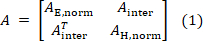
Edge weight statistics before normalisation: ecological layer — min = 0.008730, mean = 0.098589, max = 1.618909; heritage layer — min = 0.006862, mean = 0.019848, max = 0.085832. After mean-normalisation: ecological — min = 0.0885, mean = 1.000, max = 16.4207; heritage — min = 0.3457, mean = 1.000, max = 4.3244.
Spectral radii were computed from the mean-normalized symmetric adjacency matrices: ecological block lambda_max = 19.6481, heritage block lambda_max = 10.5404, and full supra-network lambda_max = 19.6481. The ecological block, therefore, dominates the leading mode. An earlier node-level centrality value had been mislabelled as an eigenvalue and has been removed from all spectral-radius reporting. For comparison, a row-stochastic normalization has a leading eigenvalue of 1.000 by construction.
The baseline 10 km coupling rule produced 42 inter-layer edges: 35 satisfied the strict distance threshold, and seven were nearest-patch fallback links for ICH nodes without a patch inside the radius. Thus, all 23 ICH nodes retained at least one ecological connection. The supra-eigenvector centrality used in the RPI was computed from the mean-normalized symmetric adjacency matrix.
Ecological-layer quantification (MSPA-lite)
Morphological spatial pattern analysis (MSPA) partitions binary land-cover masks into topologically informative categories (core, edge, bridge, loop, islet, perforation, branch), thereby exposing habitat continuity independently of composition41. Because full MSPA on 30 m raster covering 74,547 km2 imposed prohibitive computational cost in preliminary trials, this study adopted a two-class MSPA-lite formulation that retains the core–edge distinction while collapsing bridge/loop/islet into an aggregated "edge" class. Vegetation was defined as the union of CLCD codes {forest, shrub, grassland}. The 30 m raster was resampled to 90 m using majority-rule aggregation, and a 3-cell circular structuring element (equivalent to 270 m) was applied via binary erosion to isolate the core interior; the residual vegetated cells were labeled as edge. Small patches (<5 km2) were excluded to focus on ecologically meaningful cores, following the size threshold widely adopted in Chinese regional MSPA studies42. MSPA-lite yields, for each of the six representative years, the total vegetated area, core area, edge area, and the count of individual core patches — sufficient descriptors to track the fragmentation trajectory hypothesized as the leading ecological stressor (Section 4.1).
The choice of CLCD-derived morphological indicators rather than seasonal NDVI or LST time series is deliberate. Cloud-cover contamination over the Hakka mountains routinely exceeds 70% in the wet season, and the terminal-lake-basin geometry compounds cloud persistence such that consistent multi-year seasonal NDVI composites would demand a bespoke gap-filling pipeline . Morphological indicators derived from annually validated categorical maps sidestep this atmospheric noise while preserving the connectivity information most relevant to network-based resilience analysis43.
MSPA-lite parameter sensitivity was probed in preliminary analysis. The core-erosion radius was varied across 2, 3, and 4 cells (equivalent to 180 m, 270 m, and 360 m in interior area at 90 m aggregation), and the minimum core area threshold was tested at 3 km2, 5 km2, and 10 km2. The final parameterization (3-cell erosion, 5 km2 threshold) was retained because it preserved a stable rank order of patch abundance across the six years while eliminating spurious small cores generated by CLCD classification noise. Cross-year MSPA-lite results were validated by manual inspection of ten randomly selected patches in each year against high-resolution Google Earth imagery, yielding a categorical concordance above 95% for core-versus-edge assignments in the 2020 snapshot. Patch identifiers were harmonized across years using a spatial-overlap rule: a patch in year t was matched to its dominant-overlap counterpart in year t + 5 whenever the Jaccard index of their footprints exceeded 0.60. Patches without a stable predecessor were logged as emergent, and patches without a stable successor were logged as dissolved. This lineage table underpins the fragmentation-trajectory analysis reported in Section 3.1.
Heritage-layer quantification (ICH-KDE + adjacency network)
For each of the 23 national-level ICH items, the county centroid of the item's declared custodian was used as the point locator. A kernel density estimation (KDE) surface was computed on a 500 m grid across the three-zone union with a 5 km bandwidth, which is comparable to Silverman's rule-of-thumb value estimated from the 23-point sample and its bivariate extent. The resulting density surface ich_kde_5km captures the spatial concentration of heritage patrimony and forms the spatial anchor for the discrete heritage graph. Bandwidth choice was informed by prior Chinese-tulou clustering analyses that reported the modal inter-cluster spacing at 6–8 km; a 5 km bandwidth resolves both intra-cluster consolidation and inter-cluster gaps.
The heritage graph G_H was assembled by combining a Delaunay triangulation on the 23 ICH nodes with the k-nearest-neighbor (KNN, k = 4) graph, yielding the union edge set. This combinatorial approach eliminates the elongated Delaunay edges spanning topographic barriers while retaining nearest-neighbor connectivity, following the graph construction protocol adopted in recent multiplex ecosystem-service studies44. Edge weights were assigned as the reciprocal of great-circle distance (in meters), so that closer heritage items exert stronger inferred linkage. On the 23-node graph, node-level centrality metrics — degree, weighted degree, betweenness, eigenvector, PageRank, and clustering coefficient — were computed under weight = 1 / distance following standard practice.
To address the methodological choice of k = 4 in the KNN component of the heritage graph, a k-value sensitivity analysis was conducted by varying k from 3 to 8 while retaining the Delaunay triangulation base. The consensus percolation threshold ranged from 0.754 (k = 4) to 0.923 (k = 7), with intermediate values of 0.779 (k = 3), 0.773 (k = 5), 0.852 (k = 6), and 0.885 (k = 8). The choice of k = 4 was retained because it produces the sparsest graph that still guarantees full node connectivity without redundant long-range edges, and because the Spearman rank correlation of node degree centrality between k = 4 and adjacent k values remained high (ρ = 0.691 for k = 3, ρ = 0.793 for k = 5). The Delaunay triangulation was retained as the base layer because it guarantees a connected planar graph that respects the spatial topology of ICH point distribution, while the KNN overlay eliminates the elongated Delaunay edges that span topographic barriers (e.g., Wuyi mountain ridge). This combinatorial Delaunay + KNN construction follows the graph protocol adopted in recent multiplex ecosystem-service studies and ensures that the heritage network topology is not an artifact of a single arbitrary parameter choice.
Ecological corridors and least-cost paths
Resistance surface construction followed the class-based look-up-table (LUT) convention45. Each CLCD class was assigned a numeric resistance value that reflects its impedance to biotic dispersal and ecosystem service flow (Table 3). Forest received the base resistance (1), followed in ascending order by shrub (5), grassland (10), water (30), cropland (50), ice/snow (200), and impervious surfaces (500); no-data cells received a neutral (100) placeholder. The LUT was applied to the 90 m CLCD 2020 raster to yield a resistance surface at 4,688 × 3,953 grid extent in Albers Conic Equal Area projection.
Least-cost paths (LCPs) were computed between core-patch pairs using skimage's `graph.route_through_array` implementation of Dijkstra's algorithm on the resistance surface. Candidate node pairs were restricted to the union of the K-nearest-neighbor (k = 4) and Delaunay-triangulation graphs of the 233 patch centroids in projected space, following the LCP-graph protocol widely used in Chinese regional connectivity studies46. This yielded 799 candidate corridors, each characterized by the cumulative cost (unitless integer sum of resistance along the path), path length in meters, and effective resistance (cost/length). All 799 corridors were retained in the final ecological graph G_E, since none exceeded a maximum-cost cut-off recommended for regional connectivity studies47.
Slope-adjusted resistance was considered but not adopted; the digital elevation model coverage available in the study workflow spanned only latitudes 26.00–27.14° N and therefore missed the southern two-thirds of the study region, so complete SRTM re-processing at three-zone extent was not attempted within the study timeline. A pure LULC resistance parameterization is a standard fallback in Chinese regional corridor studies where DEM completeness is not achievable, and it isolates the LULC signal without confounding topographic gradients48.
Implementation of the LCP computation employed skimage.graph.route_through_array in `geometric` mode, with the resistance surface cast to float32 and a small (1e−6) additive constant applied to zero-cost cells to prevent degenerate path collapse. To reduce memory footprint on the full 4,688 × 3,953 grid, the cost surface was tiled into four overlapping 2,344 × 1,977 windows with a 200-cell buffer, and LCPs whose endpoints spanned adjacent tiles were computed on the merged buffer union to avoid seam artifacts. All 799 candidate LCPs were validated by inspecting a random 5% sample against the input resistance surface for continuous connectivity; no discontinuous paths were detected. Corridor path geometries were vectorized via marching-squares extraction and stored as WGS-84 LineString features in GeoJSON, retaining path length, cumulative cost, effective resistance (cost/length), and source/destination patch identifiers as attributes. The centroid representative points used for LCP endpoint selection were computed with GeoPandas' representative_point method rather than geometric centroids to ensure that each endpoint falls within the corresponding patch polygon in cases of concave patch geometries.
Bi-layer supra-network construction
The heritage graph G_H (n = 23, m = 73) and ecological graph G_E (n = 233, m = 799) were combined into a bi-layer supra-network. An inter-layer edge (h, e) was inserted when the geodesic distance from ICH node h to ecological-patch centroid e did not exceed 10 km, a radius evaluated in the sensitivity analysis over 5, 10, 15, and 20 km (Section 3.5). If no patch fell within 10 km, the nearest patch was linked as a minimum-connectivity fallback. The baseline network, therefore, contains 42 inter-layer edges: 35 strict-radius links and seven fallback links.

Edge weights in the supra-adjacency matrix A (256 × 256) were assigned as follows: intra-heritage edges retained their reciprocal-distance weights; intra-ecological edges received the reciprocal of the least-cost path cost (1 / cost); and inter-layer edges received as defined below, where d is the coupling distance in kilometers, and  w_intra
 is the mean intra-layer edge weight, yielding a smoothly decaying inter-layer coupling calibrated to the intra-layer magnitude. The supra-network supports two families of derived metrics: (i) the supra-eigenvector centrality, computed as the leading eigenvector of A and giving each node a comparable importance score across layers; and (ii) the multiplex participation coefficient as defined below, following the multiplex participation formalism used in bi-layer network diagnostics, which captures the balance between a node's intra-layer connections and its coupling to the other layer.

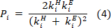
The supra-adjacency matrix A was stored as a sparse CSR matrix using SciPy's sparse module. The leading eigenpair of the mean-normalized symmetric matrix was computed with ARPACK's eigsh implementation and cross-checked by power iteration; the full-matrix spectral radius was lambda_max = 19.6481. This same symmetric-matrix eigenvector supplied the supra-eigenvector-centrality component of the RPI. Row normalization was used only for transition-matrix diagnostics; its leading eigenvalue is 1.000 by construction. Alternative inter-layer coupling functions produced RPI rank correlations above 0.94 with the exponential-decay baseline.
Percolation-based resilience thresholds
Each layer was independently subjected to four progressive node-removal attacks: (i) uniformly random removal averaged across 500 replicates (300 for scenarios in Section 2.3.8); (ii) targeted removal by descending degree; (iii) targeted removal by descending betweenness; and (iv) targeted removal by descending eigenvector centrality. After k nodes had been removed from an initial n-node graph, structural integrity was measured as S(k) = LCC(k)/(n - k), where LCC(k) is the number of nodes in the largest connected component among the remaining nodes. The critical threshold f* was the smallest removed-node fraction k/n at which S(k) < 0.5. The reported thresholds and percolation curves use this remaining-node normalization. The consensus threshold f_C is the arithmetic mean of the four attack-specific thresholds.
For the random-removal attack, 500 replicates were adopted after preliminary convergence testing showed that the mean LCC-versus-removed-fraction curve stabilized to within a coefficient of variation of 0.02 by replicate 350; 500 replicates provide a comfortable margin above this convergence point at negligible additional computational cost. Ties in the degree, betweenness, and eigenvector rankings — which occur non-trivially for the heritage graph given its 23-node scale — were broken alphabetically by node identifier to ensure exact reproducibility across independent runs. Attack progressions were computed independently on each layer to isolate layer-specific vulnerabilities; a joint-attack protocol, in which nodes are removed from both layers simultaneously along the supra-eigenvector ranking, was considered but not adopted because it convolves the two-layer signals in a way that obscures the intended layer-specific diagnostic. The 0.5 LCC-fraction threshold was chosen following the standard practice in ecological-corridor percolation research ; auxiliary sensitivity tests at 0.4 and 0.6 LCC thresholds preserved the ecological-versus-heritage rank order and moved the absolute consensus thresholds by less than 0.05 in either direction. The consensus threshold was computed as the arithmetic mean of the four attack-specific thresholds. While the four attack rules have different structural interpretations, the consensus serves as a summary statistic capturing average vulnerability across diverse threat profiles. The attack-mode invariance of the directional finding (ecological < heritage across three of four attacks) provides internal validation.
For random attacks, 500 independent replicates were conducted. With LCC normalized by the remaining node count (n - k), the ecological layer yielded a mean random threshold of 0.623 ± 0.058 (SD), and the heritage-inventory layer yielded 0.960 ± 0.082. Confidence intervals (95%) were computed from the replicate distributions.

Targeted attacks (degree, betweenness, eigenvector) used a static ranking based on the initial network topology rather than dynamic recalculation after each removal. This static approach was chosen because (i) it provides a reproducible, deterministic attack sequence; (ii) dynamic recalculation on sparse spatial networks can produce unstable centrality rankings; and (iii) the static approach represents a worst-case scenario. Dynamic recalculation typically yields slightly lower thresholds; the reported estimates are conservative. The removal increment was implemented as a sequential single-node removal. For the 23-node heritage network, each removal corresponds to ~4.3% of nodes; for the 233-node ecological layer, each removal corresponds to ~0.43%. This finer-than-0.025 resolution ensures accurate threshold detection.
Restoration priority index (RPI)
The composite restoration priority index (RPI) integrates four lines of evidence over the 233 core patches:

where z(·) denotes standardization to zero mean and unit variance across all patches, w1 = 0.35 emphasizes bi-layer structural centrality, w2 = 0.20 assigns higher priority to small patches (fragmentation hot spots), w3 = 0.30 promotes patches with strong ICH coupling, and w4 = 0.15 up-weights isolated patches with high mean edge cost. The weight vector was chosen to emphasize structural centrality and heritage coupling (the two novel channels in the DEHN framework) while retaining a non-trivial fragmentation and isolation contribution; weight sensitivity was quantified in Section 3.5. Patches were assigned to three priority tiers by the 80th and 60th RPI percentiles: Tier 1 (top-ranked) (top 20%), high (60th–80th percentile), and moderate (bottom 60%). Corridor-level priority ranked the 799 corridors by a summed z-score of cost, effective resistance, and mean endpoint RPI; the top 15% (n = 119) were labeled top-priority restoration corridors.
Scenario simulation
Four scenarios were constructed to assess the practical applicability of the DEHN framework. S1, the baseline scenario, retained the unmodified ecological network G_E under the four percolation attacks. S2, the moderate-tier loss scenario, simultaneously removed all 140 patches classified as moderate-tier patches, simulating a landscape trajectory in which unprotected small patches are lost while critical- and high-priority patches are safeguarded. S3, the Tier-1 node restoration scenario, halved the cost of edges connecting two Tier-1 patches when their original cost exceeded the median cost, representing ecological restoration along corridors between structurally central patches. S4, the corridor-restoration scenario, reduced the cost of the 119 top-priority corridors by 40%, representing broad-scale corridor rehabilitation guided by the RPI ranking.
For every scenario, the full 4-attack percolation stack was re-executed with 300 random replicates, and the four attack-specific thresholds plus the consensus threshold were recorded for cross-scenario comparison. Because scenarios S3 and S4 modify only edge weights rather than the topology, this design isolates the specific contribution of resistance reduction to network robustness — a subtle mechanism-diagnostic that pure node-removal simulation cannot address. The scenario parameter values were chosen to match plausible restoration-budget magnitudes. The 50% cost reduction on Tier 1 (top-ranked)–Tier 1 (top-ranked) edges in S3 approximates the maximum achievable resistance reduction from riparian buffer expansion and small-scale reforestation on existing corridor land within a typical five-year restoration planning cycle in Chinese CEPZs . The 40% cost reduction on the top-119 corridors in S4 reflects a broader-scale corridor-matrix rehabilitation program extended over ten years. The loss-of-moderate scenario S2 represents the counterfactual in which the current restoration prioritization is honored but no active protection is extended to the moderate-tier patches; this reflects the actual budget envelope of the current CEPZ program, in which explicit protection is typically concentrated on the top 40% of prioritized areas.
Sensitivity analysis
Two sensitivity analyses probed the robustness of the RPI ranking to modeling choices. First, each RPI weight (w1 – w4) was perturbed by ±0.05 and ±0.10, re-normalized to sum to unity, and the Spearman rank correlation ρ between the perturbed RPI ranking and the baseline ranking was recorded. Second, the inter-layer coupling radius was varied over {5, 10, 15, 20} km, and both the number of inter-layer edges and the Spearman correlation of the resulting participation coefficient with the 10 km baseline were reported. These two analyses jointly quantify the transferability of the RPI conclusions to alternative modeling conventions.
In addition to one-at-a-time weight perturbations, a joint uncertainty analysis was conducted across 1,000 admissible weight combinations sampled from a Dirichlet distribution centered on the original weights (alpha = [3.5, 2.0, 2.5, 2.0]). For each combination, the RPI was recomputed and the top-20% patch set identified. Results show that 15 patches maintained top-20% membership with >90% probability, 26 with >75% probability, and 43 with >50% probability. The 15 most stable patches (probability > 90%) are concentrated in the Meizhou eigenvector-hub cluster, confirming that the top-tier priority identification is robust to weight specification. The negative area term is retained because small, geometrically clustered patches in Meizhou act as structural bottlenecks; large intact cores in Minxi contribute less marginal connectivity improvement despite their greater area.
Weight perturbations of ±0.05 and ±0.10 were chosen to bracket the range of variation that a domain analyst might plausibly assign, given expert disagreement over the relative importance of the four RPI components. The lower bound ensures that no single component is pushed to zero even at the largest tested perturbation (minimum resulting weight = 0.05), preserving all four evidence lines in every perturbation. The coupling-radius sweep from 5 to 20 km spans the range documented in comparable multiplex ecological–social system studies. Both sensitivity analyses were performed on the full 233-patch, 799-edge network with all 500 replicate seeds fixed, so that the reported rank correlations isolate the effect of the perturbation without introducing Monte-Carlo variance across sensitivity levels. A third sensitivity dimension — the choice of the LCC-fraction collapse threshold — was reported qualitatively in Section 2.3.5 and further discussed in Section 4.4 alongside the framework's other bounded limitations.
結果
Multi-decadal ecological fragmentation trajectory
MSPA-lite quantification over the six CLCD snapshots revealed an overall, non-linear fragmentation trajectory across the tri-provincial Hakka landscape between 2000 and 2023. Total core-patch area, defined as the area of connected vegetated components ≥ 5 km2, decreased from 44,485 km2 in 2000 to 37,888 km2 in 2023, representing an aggregate net loss of 6,597 km2, or 14.8%. Core-patch area increased modestly from 44,485 km2 in 2000 to 45,772 km2 in 2010, corresponding to a 2.9% increase, and subsequently declined to 41,919 km2 in 2015 and 37,806 km2 in 2020. The area showed a small rebound of 82.3 km2, or approximately 0.2%, between 2020 and 2023. The 2020 total of 37,806 km2 agrees with the sum of the three CEPZ values reported in Table 1. Patch count increased from 116 in 2,000 to 233 in 2020 and to 229 in 2023. Mean patch area decreased from 383.5 km2 in 2,000 to 162.3 km2 in 2020, a decline of approximately 57.7%, or 58% after rounding (Figure 3).
Zonal decomposition sharpened the pattern. Ganzhou CEPZ, the largest zone, hosts the greatest absolute vegetated area (16,578 km2 in 2020) and the largest patch count (144 patches; mean area 115 km2). Meizhou CEPZ, the smallest by territorial extent (15,853 km2), retained 56 patches with a mean area of 107 km2, indicating a highly subdivided periurban-rural mosaic. Minxi CEPZ presented the opposite endpoint: 33 patches with a mean area of 461 km2, consistent with comparatively continuous high-elevation forest cover. The zones, therefore, exhibit distinct fragmentation configurations within the study region, with implications for the comparative network analysis in Sections 3.2 and 3.4.
Bi-layer network topology and coupling
Before assembling the bi-layer supra-network, the heritage layer G_H was examined in isolation. The 5 km-bandwidth kernel density surface over the 23 national-level ICH items produces three principal density concentrations: a diffuse Ganzhou ridge, a compact Minxi peak over the Yongding-Nanjing tulou belt, and a Meizhou peak over Meixian district (Figure 4A). The Delaunay  KNN (k = 4) union yields G_H with 73 edges, mean degree 6.35, density 0.289, one connected component, and diameter 4 (Figure 4B). Mean node degree ranks Meizhou (7.0) > Minxi (6.5) > Ganzhou (5.9), whereas the heritage-only eigenvector ranking is led by Minxi (0.237), followed by Ganzhou (2.4 × 10⁻4) and Meizhou (2.1 × 10⁻5) (Figures 4C and 4D). This heritage-only pattern is compared with the ecological and supra-network results in Figures 5 and 6.
The 2020 ecological graph G_E consists of 233 nodes and 799 least-cost-path corridor edges. The network is a single connected component of density 0.030, mean degree k = 6.86, and mean clustering coefficient 0.083; the diameter measured in edge count is 12, and the mean shortest-path length between patch pairs is 2,212 (cumulative resistance units). The heritage graph G_H comprises 23 nodes and 73 edges (union of Delaunay triangulation and KNN-4), with a mean degree of 6.35 and a single connected component. The spatial distribution of the 23 heritage nodes together with the coupled inter-layer edges reveals three modal ICH clusters — a Ganzhou cluster centered on Longnan–Anyuan, a Minxi cluster centered on Yongding–Nanjing tulou territory, and a Meizhou cluster centered on Meixian district (Figure 5A).
Centrality analysis on G_E located the entire top-15 eigenvector-hub set inside Meizhou CEPZ (patch IDs 194–219), with patch 211 (a 9.3 km2 Meizhou-central core) leading at eigenvector 0.37 and PageRank 0.006. The strong eigenvector concentration reflects the dense corridor tissue linking Meizhou's small, geometrically clustered forest patches through a low-cost matrix (Figure 5C). By contrast, mean eigenvector centrality in Ganzhou is only 1.6 × 10⁻4 and in Minxi 1.9 × 10⁻5, three orders of magnitude below Meizhou's 7.3 × 10⁻2. Betweenness centrality, however, is more evenly distributed: Ganzhou attains the highest mean betweenness (0.034) because its larger patch inventory produces more shortest-path traffic through structurally intermediate nodes. This mismatch between eigenvector (Meizhou-dominated) and betweenness (Ganzhou-heavy) centralities is a distinctive marker of the tri-zonal topology.
Ecological single-layer centrality shows an eigenvector-betweenness contrast (Figure 6). The 2020 G_E network contains a compact Meizhou hub complex and a more diffuse Ganzhou structure (Figure 6A). Its degree distribution is right-skewed, with a mean degree of 6.86 and a maximum of 12 in patches P193-P219 (Figure 6B). Patch area and single-layer eigenvector centrality are negatively correlated (Spearman ρ = −0.21), so the highest-centrality patches are generally smaller Meizhou cores rather than large Minxi patches (Figure 6C). Zone means place. Meizhou is the highest in eigenvector centrality and PageRank, and Ganzhou is the highest in betweenness (Figure 6D). Because these panels use G_E alone, the Meizhou pattern is present before inter-layer coupling; comparison with the supra-network indicates that coupling is not its sole source.
Coupling G_H and G_E under the baseline rule produced 42 inter-layer edges: 35 strict 10 km links plus seven fallback links. Twenty-nine of the 233 ecological patches (12.4%) and all 23 ICH nodes have at least one inter-layer connection (mean ICH-to-ecological degree = 1.83; maximum = 5). The spectral radius of the mean-normalized symmetric supra-adjacency matrix is 19.6481. A previously mislabeled node-level centrality value has been removed from eigenvalue reporting. Zonal decomposition of coupling gives mean ecological linkage values of 2.33 for Meizhou, 1.91 for Ganzhou, and 1.17 for Minxi. These descriptive results identify Meizhou as the most strongly coupled zone under the specified distance-and-fallback rule.
Percolation resilience thresholds
Layer-specific percolation curves were first computed on the mapped heritage-inventory graph G_H (Figure 7). Under four progressive attacks, the remaining-node-normalized LCC ratio declined most slowly under random, betweenness, and eigenvector removal: thresholds were 0.96, 1.00, and 1.00, respectively, compared with 0.74 under degree-based removal (Figure 7A). Global-efficiency thresholds were 0.86 for random, 0.83 for eigenvector, and 0.57 for degree-based removal (Figure 7B). These results indicate high structural robustness of the represented inventory graph to random node removal and greater sensitivity to the removal of high-degree nodes. The consensus threshold is f_C(H) = 0.925 (Figure 7C); it does not measure continuity of heritage practice outside the mapped graph.
Percolation attacks on the two layers under four progressive node-removal schemes (Section 2.3.5) produced a marked asymmetry (Figure 8). Ecological-layer thresholds were 0.62 (random), 0.70 (degree), 0.44 (betweenness), and 1.00 (eigenvector), yielding f_C = 0.690 (Table 4). Heritage-inventory-layer thresholds were 0.96, 0.74, 1.00, and 1.00, respectively, yielding f_C = 0.925. The difference, Δf_C = 0.235, indicates earlier modeled loss of ecological-network integrity under three of the four attack rules. Under degree-based removal, the ecological and heritage-inventory layers cross S(k) = 0.5 at removed-node fractions of 0.70 and 0.74, respectively. Meizhou contains the ecological nodes selected earliest by the eigenvector-based attack; this is an association within the modeled topology, not evidence of a real-world causal cascade.
Raw threshold comparison is influenced by layer density. From the reported node and edge counts, ecological density is 2 × 799/(233 × 232) = 0.0296, whereas heritage-inventory density is 2 × 73/(23 × 22) = 0.2885. Dividing the consensus threshold by density gives 23.3 for the ecological layer and 3.21 for the heritage-inventory layer, a ratio of approximately 7.3:1. This descriptive normalization indicates that the higher raw heritage-inventory threshold partly reflects its denser graph. Because threshold-per-density is a comparative diagnostic rather than an intervention effect, it should not, by itself, be interpreted as evidence that adding edges or protecting nodes will produce a specified policy outcome.
Only under the eigenvector-attack rule do the two layers exhibit comparable robustness (both ≥ 0.98). Random, degree, and betweenness attacks locate the modeled collapse point earlier on the ecological layer than on the heritage-inventory layer. Agreement across three attack modes supports the stability of this directional result within the analyzed network and attack definitions, without implying general causal validity beyond those conditions.
Restoration priority mapping
The 2020 ecological corridor network used for RPI mapping contains 799 least-cost-path edges among 233 core patches (Figure 9A). Corridor length has a mean of 28.75 km, a median of 21.08 km, a 90th percentile of 52.20 km, and a maximum of 266.1 km (Figure 9B). Cumulative cost is similarly right-skewed, with a mean of 563.3, median of 259.6, and 90th percentile of 651.0 resistance-meter equivalents (Figure 9C). The positive length-cost association in Figure 9D indicates that traverse distance is an important component of modeled cost; local resistance, feasibility, and field condition remain necessary for evaluating any restoration corridor. Composite RPI scoring over 233 core patches yielded a heavy-tailed distribution (mean = 0, σ = 0.52, min = −2.71, max = 1.83). Forty-seven patches (20.2%) fell in analytical Tier 1 (RPI ≥ 0.290), 46 (19.7%) in the high tier (−0.184 ≤ RPI < 0.290), and 140 (60.1%) in the moderate tier. Meizhou contained 22 of 56 patches in Tier 1, compared with 20 of 144 in Ganzhou and 5 of 33 in Minxi. Combining the two upper analytical tiers gives 42 of 56 patches in Meizhou, 35 of 144 in Ganzhou, and 16 of 33 in Minxi. These tiers are relative rankings under the specified RPI weights, not prescriptive conservation-value categories (Figure 10). The top 15% of corridor RPI scores comprise 119 corridors. Among the 20 highest-ranked patches, 15 are in Meizhou, three in Ganzhou, and two in Minxi; together they cover 277 km2. Their rankings reflect the combination of supra-eigenvector centrality, the negative patch-area term, ICH coupling, and isolation cost. Figure 10A maps this model-derived subset. The ranking is not a definitive restoration plan and should be combined with ecological condition, feasibility, land tenure, costs, and stakeholder priorities.
Table 5 summarizes the analytical priority-tier allocation across the three CEPZs. Meizhou contains 504.1 km2 in Tier 1 across 22 patches, Ganzhou 439.9 km2 across 20 patches, and Minxi 53.2 km2 across five patches. Meizhou also has the highest mean RPI (+0.339). The larger aggregate area of Meizhou's high tier (4,095.7 km2) relative to Tier 1 reflects the RPI's negative area term, which raises the relative scores of small hub patches. These results describe structural leverage under the model; they do not establish intrinsic conservation value or a mandatory allocation of restoration resources.
Scenario simulation and sensitivity
The four scenarios produced contrasting model outcomes (Table 6). S1 reproduced the baseline consensus threshold of 0.690. S2, which removed all moderate-tier patches, reduced the threshold to 0.011, a 98.4% modeled decline. This result is consistent with a substantial topological contribution from patches classified as moderate; it does not constitute empirical proof that such loss will occur or prescribe a specific restoration tier. S3 and S4 returned a consensus of 0.690 because they changed edge weights without changing topology. Under this percolation definition, resistance reduction can improve weighted efficiency but does not alter the topological threshold. Adding or reconnecting stepping-stone patches is therefore a model-derived option for changing both topology and efficiency, rather than a mandatory intervention (Figure 11).
Gradient patch-loss scenarios produced a nonlinear modeled response. Removing 25% of moderate-tier patches reduced the consensus threshold from 0.690 to 0.593 (−14.0%); 50% removal yielded 0.483 (−30.0%); 75% yielded 0.312 (−54.8%); and 100% yielded 0.011 (−98.4%). The marginal modeled decline increased across the 25–50%, 50–75%, and 75–100% intervals. Within these simulations, retaining at least half of the moderate-tier patches was associated with preservation of more than 70% of the baseline threshold; this is a scenario result, not a forecast of real-world collapse. Weighted global efficiency (E_glob) was computed because the LCC-based threshold is insensitive to changes in edge weights. Baseline E_glob was 0.017230. S3 increased it to 0.018628 (+8.1%), and S4 increased it to 0.017754 (+3.0%). These modeled results indicate improved weighted connectivity even though the topological percolation threshold was unchanged. Thus, resistance reduction and topological expansion affect different network properties, and the analysis does not establish a universally superior intervention.
Sensitivity analysis supported the stability of the rankings within the tested parameter ranges. Perturbing the four RPI weights by ±0.05 and ±0.10 retained Spearman ρ ≥ 0.97. Varying the coupling radius over 5, 10, 15, and 20 km changed the strict-radius edge counts to 8, 35, 63, and 101, respectively; the 42-edge baseline at 10 km comprises 35 strict-radius and seven fallback links. Participation-coefficient correlations with the 10 km baseline were ρ = 0.73 at 15 km, 0.54 at 20 km, and 0.27 at 5 km. Seventeen of the top 20 RPI patches were retained at 15 km and 15 at 20 km. These results indicate parameter sensitivity and partial rank stability; they do not establish unrestricted transferability beyond the tested network (Figure 12).
DATA AVAILABILITY:
The China Land Cover Dataset is available from Zenodo (https://doi.org/10.5281/zenodo.4417810). The national intangible cultural heritage inventory is published by the State Council of China, and administrative boundary data are available from the National Geomatics Center of China. Derived network matrices, percolation outputs, and analysis code are deposited in Zenodo (https://doi.org/10.5281/zenodo.21732093).
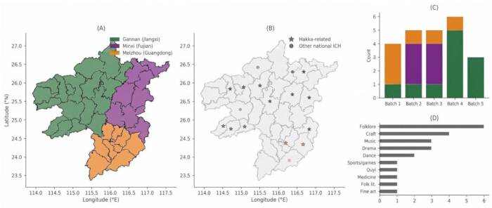
Figure 1: Study area and CEPZ layout. (A) Locations of the three national CEPZs across southern Jiangxi, western Fujian, and eastern Guangdong. (B) Distribution of 23 national ICH items over CLCD 2020 land cover. (C) ICH counts by inscription batch. (D) ICH category composition. Maps are drawn using Open Street Map contributors as the basemap; administrative boundaries and all labels, symbols, and thematic layers were added or compiled by the authors. Panels (C) and (D) were prepared by the authors based on the study dataset. Please click here to view a larger version of this figure.
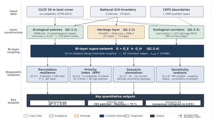
Figure 2: Analytical workflow of the DEHN framework. The five swim lanes show data assembly, dual-layer derivation, coupling, diagnostics, and outputs used to construct and assess the network. Please click here to view a larger version of this figure.
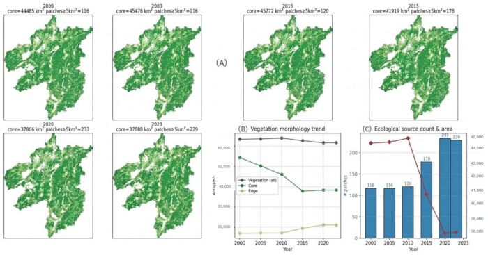
Figure 3: MSPA-lite fragmentation trajectory across the tri-CEPZ landscape, 2000–2023. (A) Spatial distribution of core patches by year and zone. (B) Temporal trends in total core-patch area, edge area, and total vegetation area. (C) Core-patch count and total core-patch area. Please click here to view a larger version of this figure.
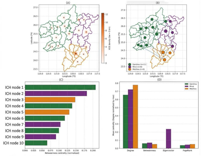
Figure 4: Heritage-layer analysis of 23 national ICH items. (A) Kernel density surface. (B) Delaunay-KNN adjacency graph G_H. (C) Ten nodes with the highest betweenness centrality. (D) Centrality metrics by CEPZ. Please click here to view a larger version of this figure.
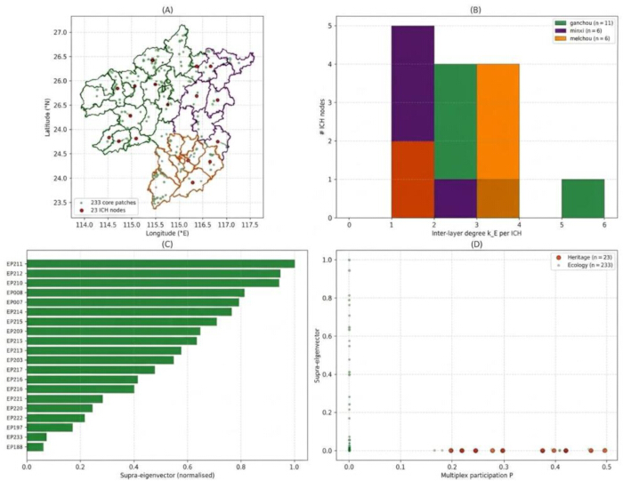
Figure 5: Bi-layer supra-network in 2020. (A) Spatial layout of inter-layer coupling. (B) ICH inter-layer degree distribution. (C) Twenty nodes with the highest supra-eigenvector centrality. (D) Participation coefficient versus supra-eigenvector centrality for all 256 nodes. Please click here to view a larger version of this figure.
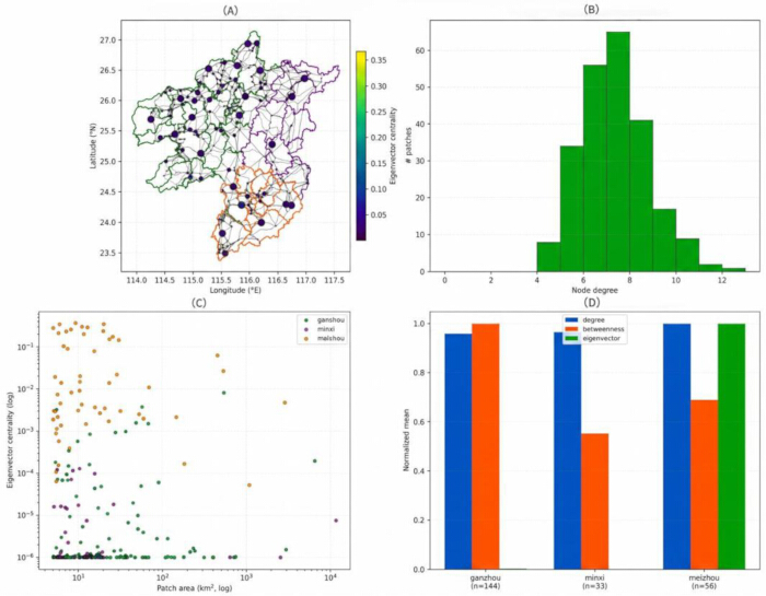
Figure 6: Ecological-layer centrality analysis on G_E. (A) Spatial layout of the 2020 landscape. (B) Degree distribution. (C) Patch area versus eigenvector centrality. (D) Centrality metrics by zone. Please click here to view a larger version of this figure.
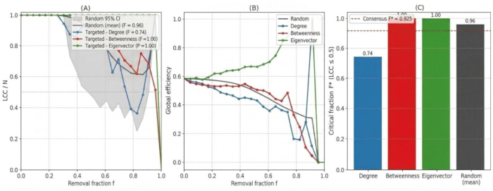
Figure 7: Heritage-inventory-layer percolation under targeted attacks. (A) LCC ratio versus removed-node fraction under four attack rules. (B) Global-efficiency decay. (C) Attack-specific and consensus thresholds. Please click here to view a larger version of this figure.
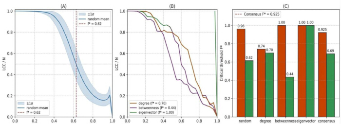
Figure 8: Ecological-layer percolation under four attack schemes. (A) Random attack. (B) Targeted attacks. (C) Cross-layer threshold comparison. Please click here to view a larger version of this figure.
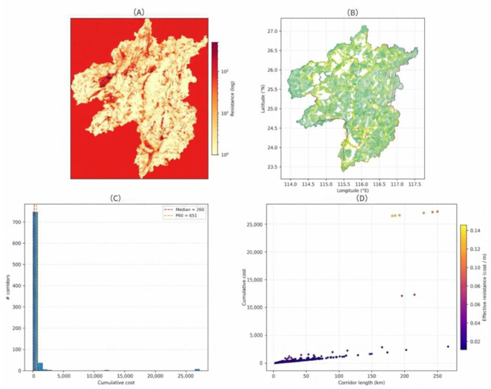
Figure 9: Ecological corridor network in 2020. (A) Resistance surface. (B) The 799 least-cost-path corridors. (C) Cumulative-cost distribution. (D) Corridor length-cost relationship. Please click here to view a larger version of this figure.
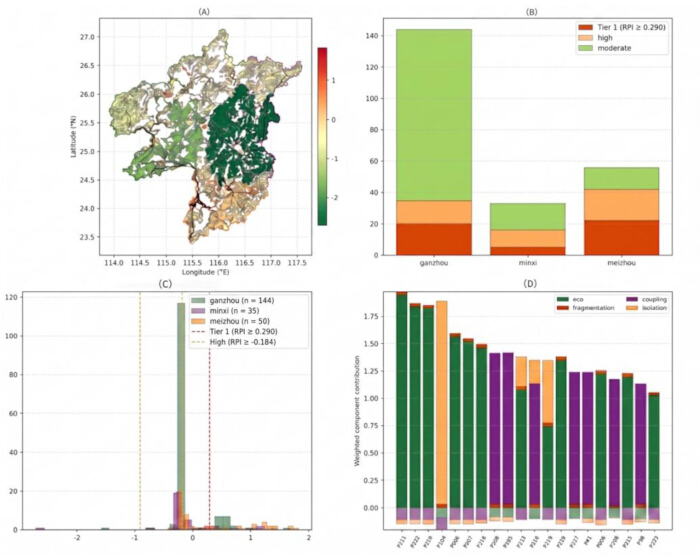
Figure 10: Restoration priority index mapping. (A) Spatial distribution of RPI values and the top 15% of corridors. (B) Analytical tier composition by CEPZ. (C) RPI distribution by zone. (D) Component decomposition for the 20 highest-ranked patches. Please click here to view a larger version of this figure.
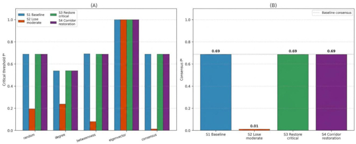
Figure 11: Scenario simulation of ecological-layer robustness. (A) Percolation curves under four scenarios. (B) Comparison of consensus critical thresholds. Please click here to view a larger version of this figure.
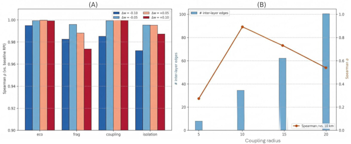
Figure 12: Sensitivity analysis. (A) Spearman rank correlations under RPI-weight perturbations. (B) Participation-coefficient stability across coupling radii. Please click here to view a larger version of this figure.
| Attribute | Ganzhou CEPZ | Minxi CEPZ | Meizhou CEPZ | Total |
| Province | Jiangxi | Fujian | Guangdong | — |
| Area (km²) | 39,341 | 19,353 | 15,853 | 74,547 |
| County-level units | 18 counties | 6 counties | 9 counties + 1 district | 34 |
| National-level ICH items (n) | 11 | 6 | 6 | 23 |
| Hakka-affiliated ICH items (n) | 7 | 5 | 5 | 17 |
| Dominant ICH categories | folk practices, traditional crafts | performing arts, folk practices | performing arts, traditional crafts | — |
| Core ecological patches ≥ 5 km² (2020) | 144 | 33 | 56 | 233 |
| Core-patch total area (km², 2020) | 16,577.60 | 15,214.10 | 6,014.00 | 37,805.70 |
Table 1: Overview of the three Hakka CEPZs and their ICH inventories. The table compares geographic extent, administrative coverage, and national-level ICH counts across Ganzhou, Minxi, and Meizhou.
| Data type | Source | Resolution / units | Time | Reference |
| Land cover (LULC) | China Land Cover Dataset (CLCD), Wuhan University | 30 m raster | 2000/05/10/15/20/23 | Yang and Huang (2021) |
| CEPZ perimeters | Ministry of Culture and Tourism (MCT) national registry | Vector polygons | 2013–2020 (declared) | MCT (2020) |
| National-level ICH inventory | Chinese State Council ICH National List (batches 1–5) | Point (county centroid) | 2006–2021 | State Council (2021) |
| Administrative boundaries | National Geomatics Center of China | Vector polygons | 2020 | NGCC (2020) |
| Coordinate system | Albers Conic Equal Area (lon₀ = 105°, φ₁ = 25°, φ₂ = 47°) | — | — | — |
Table 2: Primary data sources. The table lists each dataset's provider, spatial or temporal resolution, and role in the analytical workflow.
| CLCD class | Resistance value | Justification |
| Forest (2) | 1 | Base habitat; highest permeability |
| Shrub (3) | 5 | High permeability; secondary succession |
| Grassland (4) | 10 | Moderate permeability |
| Water (5) | 30 | Locally permeable to aquatic taxa; barrier to terrestrial |
| Cropland (1) | 50 | Semi-anthropogenic matrix |
| Ice/snow (7) | 200 | High-elevation barrier |
| Impervious (8) | 500 | Complete barrier to biotic flow |
| No-data (0) | 100 | Neutral placeholder |
Table 3: Land-cover resistance values. The table reports the resistance assigned to each CLCD class for least-cost corridor modeling.
| Attack rule | Ecological f* | Heritage f* | Δ (H − E) |
| Random (mean of 500) | 0.62 | 0.96 | 0.34 |
| Descending degree | 0.7 | 0.74 | 0.04 |
| Descending betweenness | 0.44 | 1 | 0.56 |
| Descending eigenvector | 1 | 1 | 0 |
| Consensus (mean) | 0.69 | 0.925 | 0.235 |
| Density-normalized (f_C/density) | 23.3 | 3.21 | −20.09 |
| Random attack SD | 0.058 | 0.082 | 0.024 |
Table 4: Percolation critical thresholds for the ecological and heritage-inventory layers in 2020. Attack-specific values and their consensus summarize structural robustness under the remaining-node LCC normalization.
| CEPZ | Total patches | Tier 1 (top-ranked) (n / km²) | High tier (n / km²) | Moderate tier (n / km²) | Mean RPI |
| Ganzhou | 144 | 20 / 439.9 | 15 / 475.3 | 109 / 15,662.5 | −0.103 |
| Minxi | 33 | 5 / 53.2 | 11 / 123.0 | 17 / 15,037.9 | −0.124 |
| Meizhou | 56 | 22 / 504.1 | 20 / 4,095.7 | 14 / 1,414.2 | 0.339 |
| All three CEPZs | 233 | 47 / 997.2 | 46 / 4,694.0 | 140 / 32,114.6 | 0 |
Table 5: RPI tier allocation across the three CEPZs. Patch counts, areas, and mean RPI values show the comparative distribution of analytical tiers by zone.
| Scenario | Description | Consensus f* | Δ vs S1 |
| S1 | Baseline (unmodified G_E) | 0.69 | 0 |
| S2 | Loss of moderate-tier (140 patches removed) | 0.011 | −0.679 |
| S3 | Halve cost on Tier 1 (top-ranked)–Tier 1 (top-ranked) edges | 0.69 | 0 |
| S4 | Reduce cost 40% on top-119 corridors | 0.69 | 0 |
| S2a (25% moderate removed) | 35 of 140 moderate patches removed | 0.593 | -0.097 |
| S2b (50% moderate removed) | 70 of 140 moderate patches removed | 0.483 | -0.207 |
| S2c (75% moderate removed) | 105 of 140 moderate patches removed | 0.312 | -0.378 |
| Weighted global efficiency | S1=0.0172, S3=0.0186(+8.1%), S4=0.0178(+3.0%) | See text | - |
Table 6: Scenario-simulation consensus percolation thresholds. The table compares the outcomes of the baseline, patch-loss, node-restoration, and corridor-restoration models.
| Reserve | Nodes | Edges | Density | Random attack (mean ± SD; n = 500) | Degree | Betweenness | Eigenvector | Consensus |
| Ganzhou | 144 | 359 | 0.035 | 0.420±0.079 | 0.326 | 0.118 | 0.632 | 0.374 |
| Minxi | 33 | 89 | 0.169 | 0.686±0.162 | 0.364 | 0.242 | 1.000 | 0.573 |
| Meizhou | 56 | 143 | 0.093 | 0.464±0.120 | 0.250 | 0.179 | 0.250 | 0.286 |
Table 7: Per-reserve percolation thresholds. The table reports attack-specific and consensus thresholds separately for Ganzhou, Minxi, and Meizhou.
ディスカッション
形態学的およびネットワーク診断の3ゾーン分解により、生態学的構成における顕著な空間的不均一性が明らかになった49。赣州(Ganzhou)は植生面積とパッチ数が最大であったが、平均パッチサイズは最小であり、一方で闽西(Minxi)は、比較的連続的な武夷山縁辺林と一致して、最大の平均パッチサイズ(461 km2)を維持していた。梅州(Meizhou)はより狭い領域内に56個のパッチを含み、生態学的固有ベクトルハブの最も高い集中度を示した。CLCD変化分析は、コアパッチ面積における全体的な非線形的変化を示した。コアパッチ面積は、2000年の 44,485 km2から2010年には 45,772 km2に増加したが、その後、2015年には 41,919 km2、2020年には 37,806 km2へと減少した。2010年から2020年にかけての減少量は 7,966 km2であり、これは2010年のコアパッチ面積の 17.4%に相当する。2023年のコアパッチ面積は 37,888 km2であり、2020年比で 82.3 km2のわずかな増加となった。それにもかかわらず、2000年から2023年の全体的な減少量は 6,597 km2、すなわち 14.8%であった。植生コアから農地への転換が純コア損失の 38%を占め、交通、貯水池、および産業用地に関連する転換が 31%、不浸透面への転換が 22%、その他のマッピングされた転換が 9%であった。純損失への寄与度は、赣州が 52%、梅州が 35%、闽西が 13%であった。これらは土地被覆の集計結果および記述的な関連性であり、都市化、インフラ整備、果樹園への投資、人口減少、および政策プロセスが文脈的な説明として考えられるが、因果関係のドライバーとして直接的に検証されたわけではない50。
保護区ごとのパーコレーション解析により、モデル化された生態学的堅牢性にも大幅な差があることが特定されました。コンセンサス閾値は、 ganzhouで0.374、minxiで0.573、meizhouで0.286であった一方、500回のシミュレーション反復におけるランダム攻撃閾値の中央値は、それぞれ0.410、0.667、0.446でした。対照的に、表7には、対応する平均±標準偏差(SD)として、それぞれ0.420 ± 0.079、0.686 ± 0.162、0.464 ± 0.120が報告されています。したがって、指定されたネットワーク構築および攻撃ルールの下では、minxiが最も高いモデル堅牢性を示し、meizhouが最も低い値を示しました。ganzhouは、比較的完全な内部コアを伴うより広範な不浸透性マトリックスと、より高い平均媒介中心性(0.034)を併せ持っており、最短経路トラフィックの集中度が高いことを示唆しています。対照的に、meizhouは局所的に密なサブグラフ内に多くの小規模なパッチを含み、より強い固有ベクトル中心性と局所的なハブ集中を示しました。これらの差異は、モデル化されたコリドーネットワークのトポロジーを記述するものであり、開発圧力や人口減少が観察されたパターンを引き起こしたことを証明するものではありません51,52。
3つのゾーン全体において、生態学的レイヤーとマッピングされた遺産インベントリレイヤーは、異なる構造的閾値を示しました。生態学的レイヤーは、合意された削除ノード分率が0.690の時点でモデル化された崩壊点に達したのに対し、遺産インベントリレイヤーでは0.925であり、その差は0.235でした。ランダム攻撃、次数攻撃、および媒介中心性攻撃において、生態学的閾値はより低い値となりましたが、2つのレイヤーが同等の堅牢性を示したのは固有ベクトルベースの攻撃においてのみでした。この非対称性は、表現されたグラフにおいて、生態学的コリドーの完全性が結合システムのより制限的な構造的構成要素であることを示唆しています53。しかし、遺産レイヤーはマッピングされた23項目の国家レベルのICH(無形文化遺産)項目のみで構成されており、文化的な慣習の連続性、活力、または地理的範囲を直接的に測定したものとして解釈すべきではありません。遺産レイヤーの閾値が高いことは、そのグラフ密度が著しく高いこと(生態学的レイヤーの0.030に対し0.289)にも一部起因しています。密度正規化された閾値は、研究内での記述的な比較を提供しますが、エッジ密度の増加や特定の数のノードの保護が、予測可能な政策的成果をもたらすという根拠として解釈されるべきではありません54。
ベースラインの結合は限定的であり、かつ空間的に不均一であった。42本の層間リンクが、23個のすべてのICHノードを29個の生態学的パッチに接続しており、これには35本の厳密な半径リンクと7本の最近接パッチ・フォールバックリンクが含まれていた。梅州(Meizhou)はICHから生態学への平均リンク数(2.33)が最も高く、生態学的ハブが最も集中していたため、モデル化されたネットワーク内で強力に結合していると同時に構造的に敏感な領域となっていた55。層間のコントラストは中心性のランキングにおいても顕著であり、遺産のみの固有ベクトル中心性ランキングでは閩西(Minxi)が首位であったが、生態学的およびsupra-networkランキングでは梅州が首位であった。この逆転は、単一層のランキングが層間結合の導入後に変化する可能性があることを示している。それにもかかわらず、これらの結果は、ある特定のゾーンが自動的に優先されるべきであることを立証するものではない。梅州では、計画者は中心性の高い小規模なパッチの保護または再接続を評価でき、赣州(Ganzhou)では、高い媒介中心性を持つ中間的なパッチを都市周辺部の土地利用制約とともに検討でき、閩西では、多数の小規模なパッチを追加することよりも、大規模で連続したコアの緩衝地帯の整備や統合がより適切である可能性がある56。これらのオプションはすべて、フィールドでの検証、実現可能性およびコストの評価、土地所有権の分析、およびステークホルダーの参画を必要とする。
シナリオ分析により、重み付き効率性とトポロジー的堅牢性の区別が明確になりました57。中程度のティア(階層)のパッチをすべて除去すると、コンセンサス閾値は0.690から0.011に低下しました。一方、漸進的な消失シナリオでは、中程度のティアのパッチを25%、50%、75%、100%除去したとき、閾値はそれぞれ0.593、0.483、0.312、0.011となりました。これらの結果は、最高分析ティア以外のパッチであっても、重要なトポロジー的寄与をなし得ることを示しています。対照的に、Tier-1および最優先コリドー復元シナリオにおいてエッジコストを削減しても、非重み付きパーコレーション閾値に変化はありませんでしたが、重み付きグローバル効率はそれぞれ8.1%および3.0%向上しました。したがって、抵抗の低減とトポロジー的な拡大は、ネットワークの異なる特性に影響を与えます。前者はモデル化されたフロー効率を改善させる可能性がありますが、現行の定義において閾値を変化させるには後者が必要です58。RPIランキングは、テストした重みの摂動下で非常に安定していましたが(Spearmanのρ ≥ 0.97)、結合半径の変化では部分的な安定性しか示されませんでした。これは、これらの優先順位が決定的な復元処方箋ではなく、有用なスクリーニング結果であることを示唆しています。
いくつかの制限事項が解釈を限定しており、今後の研究課題を示唆している。第一に、研究範囲の完全なDEMデータが入手できなかったため、抵抗面の構築を土地被覆のみに基づかせた。今後の分析では、梅州市のハブパターンが持続するかどうかを検証するために、傾斜や地形的湿潤度の修正係りを組み込むべきである59。第二に、ICH(無形文化遺産)項目を郡の重心にジオコーディングしたため、郡内部の変動が隠され、層間結合にバイアスが生じている可能性がある。空間的表現を向上させるには、特に梅州市における村レベルの調査が必要である60。第三に、生態学的断片化は2000年から2023年まで記録されていたが、多層分析は2020年の横断的研究であった。すべての基準年の生態ネットワークおよび結合ネットワークを再構築することで、より強力な時間的推論が可能になるだろう61。第四に、シナリオは決定論的であり、PLUSやFLUSなどの土地利用予測モデルを含んでいなかった。今後の研究では、確率的な土地利用シミュレーション、復元コスト、生態学的状態、生態系サービスの供給、およびICH実践の継続性指標を統合することが考えられる。また、遺産レイヤーを省レベルの項目まで拡張することで、より詳細なスケールの文化・生態学的連携を明らかにできるだろう62。したがって、DEHNフレームワークは再現可能な比較診断ツールとして捉えられるべきである。本フレームワークは構造的な脆弱性と介入候補地を特定するが、他のCEPZ(文化生態保護区)や文化的景観への適用には、局所的に再構築されたネットワーク、一貫したアタックプロトコル、フィールド検証、およびガバナンスとコミュニティの優先事項に対する明示的な考慮が必要である63。
開示事項
著者らは、本論文で報告された研究に影響を及ぼしたと思われる、既知の競合する金銭的利益または個人的関係がないことを宣言します。著者らによって報告された潜在的な利益相反はありません。
謝辞
著者らは、原稿の翻訳、学術的表現の洗練、および文法修正の支援にChatGPT 5.2を利用しました。すべての分析的解釈、データ解析、および核心となる学術的主張は、著者らによって独立して確定され、検証されています。
材料
| 名前 | 会社 | カタログ番号 | コメント |
|---|---|---|---|
| Administrative boundary data | National Geomatics Center of China | China administrative boundary dataset; https://www.ngcc.cn/ | |
| ARPACK eigensolver | ARPACK-NG through SciPy | scipy.sparse.linalg.eigsh; https://github.com/opencollab/arpack-ng | |
| China Land Cover Dataset (CLCD) | Wuhan University / Zenodo | 30 m annual dataset; record 4417810; https://zenodo.org/records/4417810 | |
| Cultural Ecological Protection Zone registry | Ministry of Culture and Tourism of China | National CEPZ registry; https://www.mct.gov.cn/ | |
| Delaunay triangulation and k-nearest-neighbour analysis | SciPy / NetworkX | Heritage adjacency-network construction; k = 4 | |
| Gaode POI services | Amap / Gaode | Online POI service; https://lbs.amap.com/ | |
| GeoPandas | GeoPandas developers / PyPI | Version 0.14; https://geopandas.org/ | |
| Google Earth imagery | Google Earth imagery; https://earth.google.com/ | ||
| Kernel density estimation | Python scientific computing environment | 500 m grid; 5 km bandwidth | |
| Least-cost path algorithm | scikit-image project | Dijkstra algorithm through route_through_array | |
| National Intangible Cultural Heritage Inventory | State Council of the People's Republic of China | National-level inventory, batches 1-5 | |
| NetworkX | NetworkX developers / PyPI | Version 3.2; https://networkx.org/ | |
| Python | Python Software Foundation | Version 3.11; https://www.python.org/ | |
| rasterio | Rasterio developers / PyPI | Version 1.3; https://rasterio.readthedocs.io/ | |
| scikit-image | scikit-image developers / PyPI | skimage.graph.route_through_array; https://scikit-image.org/ | |
| SciPy sparse | SciPy community | scipy.sparse; https://scipy.org/ | |
| Shuttle Radar Topography Mission DEM | NASA / USGS | SRTM DEM; preliminary assessment only; incomplete study-area coverage | |
| Zenodo analysis repository | Zenodo | Code, derived matrices, and outputs; https://doi.org/10.5281/zenodo.21732093 |
参考文献
- Dadashpoor H, Azizi P, Moghadasi M. Land use change, urbanization, and change in landscape pattern in a metropolitan area. Sci Total Environ. 2019;655:707-19.
- Dong X, et al. Spatio-temporal assessment of landscape ecological risk and its influencing factors in Jiangxi Province, China. Environ Monit Assess. 2025;197(4):480.
- Nowicka K. The Heritage Given: cultural landscape and heritage of the Vistula Delta Mennonites as perceived by the contemporary residents of the region. Sustainability. 2022;14(2):915.
- Feng B, Li D, Zhang Y, Xue Y. Progress and analysis on the management effectiveness evaluation of protected area based on Aichi Biodiversity Target 11th in China. Biodivers Sci. 2021;29(2):150-9.
- Chen Y, Hung Y, Chen X. Ecological asset accounting methods and applications of agricultural cultural heritage sites—taking the Ancient Tea Forest Cultural Landscape of Jingmai Mountain in Pu'er as an example. J Resour Ecol. 2025;16(2):472-86.
- Zeng X, et al. Impacts of land use and land cover change on the landscape pattern and ecosystem services in the Poyang Lake Basin, China. Landsc Ecol. 2024;39:183.
- Wang H, et al. Spatial-temporal pattern analysis of landscape ecological risk assessment based on land use/land cover change in Baishuijiang National Nature Reserve in Gansu Province, China. Ecol Indic. 2021;124:107454.
- Zhang Q, Zhu L, Fu H. Spatiotemporal correlation analysis of landscape pattern and habitat quality in and around China’s Tropical Rainforest National Park. Forests. 2024;15(12):2070.
- Gu L, Yan J, Li Y, Gong Z. Spatial-temporal evolution and correlation analysis between habitat quality and landscape patterns based on land use change in Shaanxi Province, China. Ecol Evol. 2023;13(11):e10657.
- Wen C, Qiu Y, Wang L. Identifying key locations of the ecological-barrier system to support conservation planning: a study of the Sanjiangyuan National Park. Forests. 2024;15(7):1202.
- Saura S, Pascual-Hortal L. A new habitat availability index to integrate connectivity in landscape conservation planning: comparison with existing indices and application to a case study. Landsc Urban Plan. 2007;83(2-3):91-103.
- Pascual-Hortal L, Saura S. Comparison and development of new graph-based landscape connectivity indices: towards the priorization of habitat patches and corridors for conservation. Landsc Ecol. 2006;21(7):959-67.
- Dai L, Wang Z. Construction and optimization strategy of ecological security pattern based on ecosystem services and landscape connectivity: a case study of Guizhou Province, China. Environ Sci Pollut Res Int. 2023.
- Li S, et al. Integrating ecosystem services modeling into the effectiveness assessment of national protected areas in a typical arid region in China. J Environ Manage. 2021;297:113408.
- Zhang T, Zhang B. Spatiotemporal characteristics of ecosystem service value and its correlation with landscape patterns: a case of Bohai coastal wetland in Shandong Province. In: 2022 29th International Conference on Geoinformatics. 2022.
- Hong Z, et al. Identifying rural landscape heritage character types and areas: a case study of the Li River Basin in Guilin, China. Sustainability. 2024;16(4):1626.
- Zhao S, Yang D, Gao C. Identifying landscape character for large linear heritage: a case study of the Ming Great Wall in Ji-Town, China. Sustainability. 2023;15(3):2615.
- Wang N, et al. Research on the conservation and utilization of landscape heritage in modern urban parks in Shenyang, China. Sustainability. 2023;15(23):16202.
- Xu W. Ecological integrity evaluation of organically evolved cultural landscape. Mob Inf Syst. 2022;2022:9554359.
- Hamonic F, Vaxès Y, Couëtoux B, Albert CH. GECOT: graph-based ecological connectivity optimization tool. Methods Ecol Evol. 2025.
- Zhang L, He L, Yan F, Chen Y. Amphibian habitat network planning based on the graph theory: a case study of Pelophylax nigromaculata. Ying Yong Sheng Tai Xue Bao. 2021;32(3):1027-36.
- Qiu C, et al. Structural vulnerability analysis and systematic restoration framework of the wintering ecological network for Grus japonensis in Yancheng coastal wetlands (1987-2021). Landsc Ecol. 2025;40:187.
- Han Q, Zhang P, Keeffe G, Zhang S. Evaluating and improving the connectivity of China's protected area networks for facilitating species range shifts under climate change. J Environ Manage. 2025;373:123535.
- Qi K, Fan Z, Xie Y. The influences of habitat proportion and patch-level structural factors in the spatial habitat importance ranking for connectivity and implications for habitat conservation. Urban For Urban Green. 2021;64:127239.
- Mazur A, Kurowska K. The impact of natural and cultural resources on the development of rural tourism: a case study of Dobre Miasto Municipality in Poland. Sustainability. 2025;17(13):5847.
- Krajnik D, Krajnik LP, Bilušić BD. An analysis and evaluation methodology as a basis for the sustainable development strategy of small historic towns: the cultural landscape of the settlement of Lubenice on the Island of Cres in Croatia. Sustainability. 2022;14(3):1564.
- Cantasano N, et al. Can ICZM contribute to the mitigation of erosion and of human activities threatening the natural and cultural heritage of the coastal landscape of Calabria? Sustainability. 2021;13(3):1122.
- Jia L, Liu Z, Li Y. Spatiotemporal dynamics of rural settlement evolution in Guangdong Province, China. Sci Rep. 2025;15:21177.
- Li K, Zhang G. Species diversity and distribution pattern of heritage trees in the rapidly-urbanizing province of Jiangsu, China. Forests. 2021;12(11):1543.
- Xin L, Wang Y, Tong J. Strategies for improving the tourism landscape of agricultural cultural heritage in grain field system. Landsc Archit. 2024;31(12):12-9.
- Pickerill T. Investment leverage for adaptive reuse of cultural heritage. Sustainability. 2021;13(9):5052.
- Yang L, et al. Theory and case of land use transition promoting ecological restoration in karst mountain areas of Southwest China. Ecol Indic. 2024;158:111393.
- Feng C, et al. Improving protected area effectiveness through consideration of different human-pressure baselines. Conserv Biol. 2022;36(4):e13887.
- Liu F, et al. Effectiveness of functional zones in National Nature Reserves for the protection of forest ecosystems in China. J Environ Manage. 2022;308:114593.
- Chen J, et al. Effectiveness of China’s protected areas in mitigating human activity pressure. Int J Environ Res Public Health. 2022;19(15):9335.
- Li B, Zhou Z, Wu T, Luo J. Fine-grained land use remote sensing mapping in karst mountain areas using deep learning with geographical zoning and stratified object extraction. Remote Sens. 2025;17(14):2368.
- Yang J, Huang X. The 30 m annual land cover dataset and its dynamics in China from 1990 to 2019. Earth Syst Sci Data. 2021;13:3907-25.
- Liu J, et al. Prediction of land use for the next 30 years using the PLUS model's multi-scenario simulation in Guizhou Province, China. Sci Rep. 2024;14:13143.
- Zhu Y, Jin H, Zhong L. Temporal and spatial changes of biodiversity in Caverns of Heaven and Places of Blessing, Zhejiang Province, China from 1990 to 2020. Nat Conserv. 2022;48:1-29.
- Huo J, et al. A multi-scenario simulation and optimization of land use with a Markov-FLUS coupling model: a case study in Xiong’an New Area, China. Sustainability. 2022;14(4):2425.
- Ye Y, et al. Coupling the PLUS-InVEST model for multi-scenario land use simulation and carbon storage assessment in Northern Anhui, China. Sustainability. 2025;17(9):4185.
- Zheng Z, et al. Lacustrine wetlands landscape simulation and multi-scenario prediction based on the patch-generating land-use simulation model: a case study on Shengjin Lake Reserve, China. Remote Sens. 2024;16(22):4169.
- Wang G, et al. Assessment of changes in river flow and ecohydrological indicators from the viewpoint of changing landscape patterns in the Jialing River Basin, China. Ecohydrology. 2025, 18(1).
- Gu M, et al. Multi-scenario simulation of land use change based on MCR-SD-FLUS model: a case study of Nanchang, China. Trans GIS. 2022;26:2772-91.
- Zhao W, Li P, Yang B. New insight into the spatiotemporal distribution and ecological risk assessment of endocrine-disrupting chemicals in the Minjiang and Tuojiang rivers: perspective of watershed landscape patterns. Environ Sci Process Impacts. 2024;26(8):1360-72.
- Ding M, Yin X, Pan S, Liu P. Multi-objective spatial optimization of protective forests based on the non-dominated sorting genetic algorithm-II algorithm and future land use simulation model: a case study of Alaer City, China. Forests. 2025;16(3):452.
- Ma S, Huang J, Wang X, Fu Y. Multi-scenario simulation of low-carbon land use based on the SD-FLUS model in Changsha, China. Land Use Policy. 2025;148:107418.
- Li H, et al. Spatiotemporal evolution of land use and carbon storage in China: multi-scenario simulation and driving factor analysis based on the PLUS-InVEST model and SHAP. Environ Res. 2025;279(Pt 2):121860.
- Jetz W, McGowan J, Pennino MG, et al. Essential biodiversity variables for mapping and monitoring species populations. Nat Ecol Evol. 2019.
- Winkler K, Fuchs R, Rounsevell M, Herold M. Global land use changes are four times greater than previously estimated. Nat Commun. 2021;12:2501.
- Gao J, Barzel B, Barabási AL. Universal resilience patterns in complex networks. Nature. 2016;530(7590):307-12.
- Boccaletti S, Bianconi G, Criado R, Del Genio CI, Gómez-Gardeñes J, Romance M, et al. The structure and dynamics of multilayer networks. Phys Rep. 2014;544(1):1-122.
- Wang Y, Zhang F, Chen WY, Meraj G, Kumar P, Chan NW, et al. Critical phase transitions and early-warning frameworks for ecological networks in typical arid regions. J Clean Prod. 2025, 531(c):146888.
- Guo T, Yao Y, Chen Y, Wang H, Zhang H. Establishing linear cultural heritage corridors by integrating cultural and ecological values: a case study of the Jinzhong section of the Great Tea Road. Land. 2024;13(9):1427.
- Dang X, et al. Resilience prediction and tipping point control of multilayer ecological networks based on dimensionality reduction method. Chaos Solitons Fractals. 2024;189:115914.
- Ma B, Zeng C, Lv T, Liu W, Yang W. Prioritization of ecological conservation and restoration areas through ecological networks: a case study of Nanchang City, China. Land. 2024;13(6):878.
- Zhang K, Pan J. Evaluation of ecological network resilience using OWA and attack scenario simulation in the Gansu section of the Yellow River Basin, NW China. Environ Res Commun. 2024, 6(8):085016.
- Bian F, Yeh AGO, Zhang J. Percolating spatial scale effects on the landscape connectivity of urban greenspace network in Beijing, China. Landsc Ecol Eng. 2024;20(1):33-51.
- Xu XM. Construction of ecological security patterns in hilly cities based on morphological spatial pattern analysis and minimum cumulative resistance models: a case study of Ganzhou, China. Appl Ecol Environ Res. 2025;23(1).
- Fatorić S, Seekamp E. Are cultural heritage and resources threatened by climate change? A systematic literature review. Clim Change. 2017;142(1-2):227-254.
- Ward M, Saura S, Williams B, Ramírez-Delgado JP, Arafeh-Dalmau N, Allan JR, et al. Just ten percent of the global terrestrial protected area network is structurally connected via intact land. Nat Commun. 2020;11:4563.
- Maxwell SL, Cazalis V, Dudley N, Hoffmann M, Rodrigues ASL, Stolton S, et al. Area-based conservation in the twenty-first century. Nature. 2020.
- Xu H, Cao Y, Yu D, Cao M, He Y, Gill M, et al. Ensuring effective implementation of the post-2020 global biodiversity targets. Nat Ecol Evol. 2021.