산업 5.0의 지속 가능한 제조를 위한 설명 가능한 AI 지원 사이버-물리 협업

요약

본 연구는 MIMII 데이터셋을 기반으로 산업용 음향 이상 탐지를 위해 CNN-transformer와 SHAP을 이용한 설명 가능한 AI(Explainable AI) 기반의 Industry 5.0 사이버-물리 협업 프레임워크를 제시합니다. 엣지 컴퓨팅 통합을 통해 해석 가능하며 인간 중심적인 예측 보전을 지원합니다.

초록

In this study, we present an innovative approach to the sustainable manufacturing of industrial parts using an explainable artificial intelligence (XAI)- based cyber-physical collaboration system for Industry 5.0. Current cyber-physical human systems (CPHSs) have been found to integrate AI only to a limited extent and often lack explainability. Consequently, there is a need to improve their scalability and flexibility, in keeping with the tenets of Industry 5.0: resilience, long-term viability, and human-centricity. To address these shortcomings, we introduce an architecture that integrates deep learning and explainable AI into the Cyber-Physical System (CPS) ecosystem to enable smart, explainable decision-making. Specifically, we use the Malfunctioning Industrial Machine Investigation and Inspection (MIMII) dataset for machine fault detection from acoustic signals. Audio signals undergo spectral transformation to generate spectrogram images, which are then processed by a convolutional neural network (CNN) for spatial feature extraction and a transformer encoder for temporal features. To improve transparency and facilitate human-in-the-loop cooperation, the Shapley additive explanations (SHAP)-based approach helps operators understand the system's decision-making process by highlighting input features that influence model predictions. In addition, the framework is applied in an edge-computing-based cyber-physical system to achieve low latency and low energy consumption while providing timely responses, thereby helping ensure a sustainable production environment. Experimental findings show that the proposed CNN-Transformer architecture achieves 98.5% accuracy and outperforms existing CPHS systems while maintaining low latency. The use of explainable AI in such a cyber-physical cooperation system greatly increases operator confidence and enables seamless human-machine collaboration.

서론

The transition from Industry 4.0, which emphasized technology, mechanization, and communication, to the new Industry 5.0 model, which combines technological advancement with adaptability, sustainable development, and human-centeredness, has influenced the dynamic evolution of industrial systems^1,2. The European Commission defines Industry 5.0 as a paradigm focused not only on productivity and efficiency but also on the three pillars of human-centricity, sustainability, and resilience. It is important to note that recent research has pointed out the role of AI systems, human-machine cooperation, and sustainable manufacturing as the main drivers of Industry 5.0 environments^3,4. Traditional maintenance methods are no longer sufficient in this evolving industrial environment. To enable resilience in complex, unstable contexts, maintenance must evolve into a more adaptable and systemic form⁵. Since 2011, Industry 4.0 has been the dominant model for industrial transformation in Europe, encouraging the digital transformation of businesses to enhance operations and maximize available resources⁴. Increasing efficiency without eliminating human labor in production, while protecting workers’ health and safety, is therefore imperative. Because of this, businesses and academics have begun defining the tenets of the Industry 5.0 paradigm^5,6,7, partly motivated by the Japanese notion of Society 5.0^8,9,10,11. Despite the increased emphasis on sustainable maintenance in recent literature, most existing systematic evaluations remain fragmented or domain-specific, lacking a comprehensive framework that integrates resilience, sustainability, and AI. For example, the authors examine sustainable maintenance practices for specific systems or strategies, including sustainable total productive maintenance (STPM), whereas the researchers talk about incorporating sustainability themes into maintenance techniques^12,13,14. Author conducted a comprehensive assessment of sustainability adoption criteria and highlighted technological factors that enable manufacturing to have a positive sustainable impact¹⁵. Nevertheless, within the Industry 5.0 paradigm, sustainability, resilience, and AI-based decision-making are not fully integrated in any of these works. As a result, separate maintenance methods frequently address sustainability. SHAP stands out among other explainable artificial intelligence (XAI) techniques due to its theoretically sound feature attribution method^16,17,18.

Data-driven decision-making is enabled by AI, but accurate models often require large amounts of data. Conventional machine learning (ML) techniques, such as decision trees, logistic regression, and linear regression, frequently perform poorly in highly nonlinear situations because they assume relatively simple data distributions¹⁹. By learning intricate feature representations from massive datasets, deep neural networks (DNNs) get around these restrictions²⁰. Deeper networks often perform better than shallow structures on complex decision-making tasks, according to studies²¹, but their increasing depth and parameter complexity make the model less interpretable²².

A Cyber-Physical System (CPS) is a crucial enabling technology for Industry 5.0 manufacturing because it combines distributed intelligence, embedded computers, physical processes, and communication. To enable flexible, intelligent, and real-time industrial operations, modern CPSs are rapidly integrating edge computing, edge AI, and green Internet of Things (G-IoT)^23,24. Sustainability and resilience have been highlighted in recent studies on Maintenance 4.0 and smart maintenance. While earlier works have examined the significance of Maintenance 4.0 technology in sustainable manufacturing and suggested modeling frameworks for sustainable maintenance, bibliometric and systematic studies have assessed smart maintenance technologies^25,26,27,28. Further research has investigated the integration of sustainable maintenance into Industry 4.0 environments and sustainability-oriented production systems^29,30,31,32. The Operator 4.0 concept³³, human-centric Industry 5.0 frameworks³⁴, and socioeconomic perspectives³⁵ have all garnered significant attention to human-centric maintenance. Additionally, advancements in digital maintenance³⁶, predictive and prescriptive maintenance^37,38, and sustainable maintenance strategies^39,40 have been emphasized in recent studies. Despite these advancements, research remains dispersed, and few studies offer a cohesive paradigm that integrates explainable AI, sustainability, resilience, and human-centered cyber-physical cooperation. Cyber-Physical Systems (CPSs) have not attained full autonomy despite their growing deployment, and the Industry 5.0 paradigm does not favor it. Industry 5.0, on the other hand, places greater emphasis on human supervision, cooperation, and decision-making. By incorporating human thinking and cooperation into cyber-physical processes, cyber-human systems such as human-in-the-loop CPSs (HiLCPSs)⁴¹, Human-Centered CPSs (HCPSs)^42,43, and Cyber-physical human systems (CPHSs)⁴⁴extend traditional CPSs. This integration improves adaptability, transparency, safety, and resilience by enabling real-time collaboration between intelligent systems and human operators^45,46.

Industrial audio anomaly detection has been greatly enhanced by new architectures, including Vision Transformer (ViT), Audio Spectrogram Transformer (AST), Conformer, and self-supervised learning; however, their integration with explainable cyber-physical systems for Industry 5.0 remains limited. Without integrating explainability, edge deployment, and human-in-the-loop decision support into a single framework, current research primarily focuses on classification accuracy or on post hoc XAI-based interpretability. This study proposes a novel Explainable AI-enabled CNN-Transformer cyber-physical collaboration architecture that combines edge computing, temporal dependency modeling, SHAP-based explainability, spatial feature learning, and human-centric decision support to enable sustainable Industry 5.0 manufacturing and overcome these constraints.

Thus, there remains a substantial research deficit. Current CNN/Transformer-based acoustic anomaly detection techniques favor classification performance but lack cyber-physical cooperation and explainability. While Industry 5.0 frameworks offer conceptual human-centric models that do not integrate explainable deep learning, edge intelligence, and operator-assisted decision-making into a single system, XAI-based predictive maintenance techniques increase transparency but operate independently of CPHS architectures. Therefore, a single Industry 5.0 Cyber-physical human system that integrates precise auditory anomaly detection, SHAP-based explainability, edge-enabled deployment, and human-in-the-loop cooperation is still lacking.

This paper proposes a novel Explainable AI-enabled CNN-Transformer cyber-physical collaboration paradigm for Industry 5.0 to overcome these constraints. The suggested architecture combines edge computing deployment, CNN-based spatial feature extraction, Transformer-based temporal dependency learning, SHAP-based explainability, and human-in-the-loop decision support into a single CPHS framework. The suggested framework offers an integrated solution that concurrently enhances anomaly detection performance, model transparency, operational efficiency, and human-centric collaboration for sustainable manufacturing, in contrast to current methods that handle these elements independently.

This study's main goal is to create an Explainable AI-enabled Cyber-physical human system (CPHS) for sustainable Industry 5.0 manufacturing by combining SHAP-based explainability, edge computing, and human-in-the-loop decision support with a hybrid CNN-Transformer-based acoustic anomaly detection approach. In particular, the suggested framework aims to improve anomaly detection accuracy while providing clear, understandable forecasts, facilitating effective edge deployment, and encouraging cooperative decision-making between intelligent systems and human operators. By concurrently achieving high detection performance, explainability, low-latency operation, and human-centric cyber-physical collaboration, this integrated architecture addresses the shortcomings of current acoustic anomaly detection, XAI-based predictive maintenance, and CPHS frameworks.

The suggested architecture presents a unified Explainable AI-enabled Cyber-physical human system (CPHS) for Industry 5.0, in contrast to current acoustic anomaly detection techniques, which primarily focus on classification accuracy. Within a single architecture, it combines CNN-based spatial feature extraction, Transformer-based temporal modeling, SHAP-based explainability, edge computing, and human-in-the-loop decision support. The suggested architecture addresses key issues of transparency, operator assistance, and cyber-physical cooperation by fusing precise anomaly detection with comprehensible decision-making and real-time edge deployment. The main scientific contribution of this work is the system-level integration, which sets the suggested approach apart from previous research that focuses on anomaly detection, explainable AI, or Industry 5.0 frameworks alone.

프로토콜

The suggested methodology uses a system-based Industry 5.0 Cyber-physical human system (CPHS) approach that combines explainable deep learning with a cyber-physical collaboration framework enabled by edge computing to support sustainable manufacturing processes. First, the problem is addressed by recognizing certain limitations of current CPHS solutions, such as a lack of AI-powered intelligence, explainability, and human-centric collaboration. To address the challenges, the proposed solution leverages the MIMII dataset for industrial machine condition monitoring using acoustic signal processing.

The proposed framework begins by feeding the generated spectrograms to a CNN model that extracts spatial features by recognizing significant frequency patterns associated with different machine conditions. The extracted spatial features will be converted into sequences and fed into a transformer encoder module to capture temporal dependencies via self-attention. The transformed feature representation is subsequently passed to a fully connected classifier module to classify machine states as normal or abnormal. In addition, to ensure transparency and facilitate human-centric decision-making, the SHAP explainability approach is employed to explain predictions by selecting significant time-frequency regions in the model output. The designed model will be implemented in an edge-enabled CPS setting, enabling real-time inference with low computational latency and energy expenditure. In addition, a human-in-the-loop scheme will be integrated to enable human operators to validate using explainability results. Performance is validated using accuracy, precision, recall, and F1-score, as well as other system-level metrics such as latency and energy efficiency.

The proposed framework is an XAI-driven CPHS mechanism for sustainable manufacturing in the context of Industry 5.0, and its workflow is presented as a pipeline from data acquisition to intelligent decision-making and execution, as shown in Figure 1. In the initial stage of the data acquisition procedure, sound signals are collected from machines in industries such as motors, pumps, and bearings using datasets including MIMII. Data signals thus obtained are forwarded to the next stage, referred to as data preprocessing, where they undergo filtering, normalization, and segmentation. The segmented data signals are finally converted to a spectrogram using the short-time Fourier transform (STFT) at the feature representation layer.

Then, the AI model layer uses the spectrogram images to extract features via the CNN module, identifying spatial patterns and anomalies. Then, the extracted features are reshaped and fed into the transformer encoder, which learns temporal dependencies and long-range relationships via self-attention mechanisms. The resulting feature vectors are classified as normal or abnormal using the classification layer. To ensure transparency in the prediction process, the explainability layer uses SHAP to highlight significant time-frequency regions in the spectrogram.

Additionally, there is a human-in-the-loop process in which operators interpret and provide feedback on the model's outcomes. In the deployment layer, the model runs on an edge-based CPHS infrastructure, ensuring fast inference and low power consumption, while optionally interfacing with cloud systems for storage requirements or advanced analytics. Altogether, the framework ensures accurate fault detection, explainability, and efficient real-time operation in line with the requirements of Industry 5.0.

Problem definition and requirement analysis

Cyber-physical human systems (CPHS) in Industry 5.0 settings promise intelligence, sustainability, and human-centeredness. Still, contemporary frameworks for building CPHS are hindered by a lack of advanced AI-enabled capabilities, explainability, and adequate support for human-machine collaboration. Indeed, conventional CPHS are based on rule-based or uninterpretable models, which impede adaptation to changing industry conditions and limit the operators' confidence in automation. Moreover, conventional CPHS cannot effectively analyze highly sophisticated data, such as industrial acoustic signals containing both spatial (i.e., frequency) and time-dependent components, which are important for predictive maintenance. Hence, it is necessary to create a framework that can detect machine anomalies with high precision, provide explanations, and operate at the edge, thereby enabling CPS.

Here x(t) is the acoustic input signal, S(f,t) is the spectrogram representation of the signal,  is the label and θ is the parameter set of the CNN-Transformer architecture. Symbols used in subsequent equations are introduced right after their first appearance in order to preserve mathematical correctness.

From a mathematical point of view, the task can be formalized as a supervised learning problem. Let the industrial acoustic signal be denoted by x(t). The STFT of x(t) is computed according to the formula:

   (1)

where ω(.) is the window function and f is the frequency. The generated spectrogram  serves as the input to the deep learning algorithm. The goal is to train the mapping function

    (2)

where  is the class label (either normal or abnormal), and where S is the spectrogram input, y is the predicted output label and θ is the set of learnable parameters of the CNN-Transformer architecture. The optimization problem is formulated as the minimization of the classification loss:

  (3)

subject to the constraints of minimum latency , energy efficiency , and interpretability, wherein the explanation ∅(SHAP) captures the importance of features in the prediction process,

   (4)

where  is the contribution of each individual feature. In line with the foregoing, the design requirements include the following: (i) reliable anomaly detection based on hybrid deep learning, (ii) interpretable outputs for human intervention, and (iii) implementation in an edge-enhanced CPS framework.

Dataset acquisition and preprocessing

In this regard, to assess the proposed Explainable AI-based CPHS framework, the MIMII Dataset¹³ has been selected. This dataset is a widely used benchmark for detecting anomalies in industrial machinery using acoustic signals. This database contains sound recordings of various machines, such as slide rails, fans, pumps, and valves, under both normal and faulty operating conditions. For each machine, recordings vary with different settings and noise environments. This makes it suitable for training and evaluating models under real-time industrial conditions.

Whereas the MIMII dataset is widely used in unsupervised anomaly detection studies that rely solely on normal samples during training, it includes explicit annotations of both normal and anomalous machine states. The problem is posed as a supervised binary classification task to test the ability of the proposed Explainable AI-based CNN-Transformer architecture to separate healthy from faulty machine states. Specifically, the official MIMII labels are used, assigning class label 0 to normal samples and class label 1 to anomalous samples.

Table 1 shows the Dataset Description Details. Approximately 12,000 recordings of acoustic signals are considered in the current research, including both normal and faulty machinery operations. As per the requirements, all recordings in this study have been captured at 16 kHz and are 10 s long. Although the dataset contains approximately 12,000 recordings, a class-balanced subset of 2,000 test recordings was selected solely to visualize the confusion matrix. All reported performance metrics were computed using the complete test set (approximately 2,400 recordings). Furthermore, training and test samples are separated at an 80:20 ratio for model training. This database is well-suited for Industry 5.0 applications because it includes real-time noise conditions. The recording distribution used in this study is given in Table 2. From this dataset, approximately 12,000 recordings covering all machine types and signal-to-noise ratio (SNR) conditions were selected for the supervised binary classification experiments using an 80:20 train/test split, shows the industrial machine types, corresponding machine IDs, total numbers of normal and anomalous acoustic recordings, SNR conditions, and the experimental train/test partition employed for supervised binary classification.

The experiment was carried out using the MIMII (Malfunctioning Industrial Machine Investigation and Inspection) dataset version 1.0, which comprises four types of industrial machines: fans, pumps, valves, and slide rails. Data were collected from different machine IDs (ID00–ID06, depending on the machine type) and conditions. The MIMII database comprises data acquired at signal-to-noise ratios (SNRs) of −6 dB, 0 dB, and +6 dB. Normal data corresponds to the healthy condition of the industrial machine, while anomalous data corresponds to an anomalous condition. The classes were labeled based on the database annotation, with normal data labeled class 0 and anomalous data labeled class 1.

A fair evaluation procedure required that the split between train and test sets occur at the original audio-recording level prior to any splitting, augmentation, or spectrogram creation steps. As a result, audio segments from the same recording could not appear in both the train and test sets. For the evaluation experiment, recordings with different signal-to-noise ratios (−6 dB, 0 dB, and +6 dB) were used, which provided an opportunity to evaluate the suggested framework under various industrial conditions.

To prevent data leakage, the train/test split was performed using the original audio file as the basis, prior to any segmentation or spectrogram generation. Segments from the same 10 s audio recording were assigned exclusively to either the training or the testing set, with no segments present in both sets. Afterward, spectrograms were generated and augmented separately for each dataset. This way, the problem of data leakage is avoided, thereby preventing an overly optimistic assessment of performance.

Dataset preprocessing

The unprocessed acoustic signals from the MIMII dataset are then processed to improve signal quality and enable effective feature extraction. The input signal is denoted by x(t), where t is time. The first process is noise filtering, whereby background noises are filtered using a filtering function such that:

   (5)

where ∗ represents the convolution process and h(t) is the filter's impulse response. This process enhances the clarity of the acoustic signal and minimizes the effects of noise often prevalent in industrial environments. Signal normalization is used to ensure that the amplitudes of all audio signals are comparable before feeding them into the deep learning model. The normalized signal, denoted as x_n(t), is calculated as:

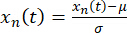   (6)

where μ and σ are the mean value and standard deviation of the input signal, respectively. All input signals are guaranteed to have zero means and unit variances thanks to this procedure. Finally, for processing, the normalized input signal is divided into multiple tiny pieces. Given that the length of the entire signal is T, it is broken down into N overlapping frames, each having a length L using a sliding window function:

   (7)

where H is the hop size. The spectrogram can be defined by the formula below:

   (8)

The spectrograms obtained in this way are fed into the CNN-transformer-based framework to extract spatial and temporal features for successful anomaly detection. Figure 2 shows the preprocessing pipeline.

Figure 2 illustrates a vertical preprocessing pipeline that may be employed for acoustic data acquired in industry. Firstly, the raw audio signals are extracted from the MIMII dataset and fed into the noise-removal stage to reduce noise. This is followed by normalizing the signal to remove amplitude inconsistencies, ensuring the signal is consistent. The signal is later split into smaller overlapping sections. Following segmentation, STFT transforms will be applied to the data to convert time-domain signals into time-frequency signals. Then, the power spectrum is calculated as part of generating the signal's spectrogram. Preprocessed spectrograms will thus be the output generated in the process and will be used in the proposed CNN-transformer model.

Spectrogram generation

After data normalization and segmentation, acoustic signals are converted into a time-frequency representation using the Short-Time Fourier Transform (STFT). The resulting spectrogram provides a pictorial representation of changes in frequency composition over the period of analysis. In industrial settings, machine faults usually manifest as frequency patterns, making spectrograms more useful for detecting machine anomalies.

The resulting processed data is therefore converted into spectrogram images to distinguish between normal and abnormal instances within the machines. The audio data will be converted into multiple spectrograms to enable the learning model to analyze local frequency components and temporal changes within the machine process. These images are used as input data for the CNN-transformer model, where the CNN handles spatial (frequency) patterns while Transformers handle temporal relationships.

Algorithm 1: Spectrogram Generation from Acoustic Signals

Input: Raw audio signal x(t)

Output: Spectrogram S(t, f)

Step 1: Load audio signal  x(t)

Step 2: Apply noise filtering

Step 3: Normalize signal x_n(t)

Step 4: Segment signal into frames:

for k = 1 to N do

end for

Step 5: Apply a window function w(t) to each segment

Step 6: Compute STFT:

  (9)

Step 7: Compute magnitude:

   (10)

Step 8: Store spectrogram S(t, f)

Step 9: Return spectrogram dataset 

The process of generating spectrograms starts with acquiring the original audio signal, followed by preprocessing steps such as noise reduction and signal normalization to ensure signal integrity and quality. After that, the normalized audio is sliced into multiple overlapping windows to capture the temporal characteristics of both long- and short-term periods. To prevent spectral leakage, each of the slices is multiplied by the window function before being passed through the Short-Time Fourier Transform. Afterward, the transformed signal is represented as a complex-valued function in the frequency domain, and its magnitudes are squared. Thus, the energy of the frequencies over the given time is represented by the spectrograms. Finally, they are stored as image-like data and fed to the neural network for training.

Spatial feature extraction using CNN

After the process of creating spectrograms, the output time-frequency images are taken as inputs and are given to a Convolutional Neural Network (CNN). Assuming the input spectrogram as , where H is the frequency domain and W is the time domain. The purpose of using the CNN here is to learn discriminative spatial features from the input spectrogram. These discriminative spatial features will help differentiate between normal and abnormal machine behavior in an industrial environment.

A basic operation performed by the Convolutional Neural Network (CNN) is convolution. Convolution with a given filter  is given as:

   (11)

The operation described above enables the neural network to identify local spatial features, such as edges, frequencies, and harmonic content, in the spectrogram. This is done through multiple filter operations that generate various feature representations, producing several feature maps. Convolution is followed by a non-linear activation function, as shown below:

  (12)

This non-linearity enables the network to capture and represent complex relationships among variables. The next stage in a convolutional neural network involves the application of pooling operations. The common technique of max pooling is expressed mathematically as follows:

   (13)

where Ω refers to the pooling window. Pooling helps to achieve translation invariance and retain only the relevant information while discarding redundancy. From low-level variables such as frequencies to complex machine behavior, higher-level features can be extracted hierarchically using a convolutional neural network. Consequently, feature maps can be used to depict the network's ultimate output:

   (14)

where represents the learnable parameters of the CNN. The feature maps contain rich spatial information and are transformed into sequences to serve as inputs to the transformer encoder in the next phase. The above-described spatial feature extraction process is crucial for enabling the model to detect minute anomalies in industrial acoustic signals.

Figure 3 demonstrates how spatial features are extracted horizontally from the spectrogram input using a CNN model. It starts with the input spectrogram, which encodes time-frequency properties of the audio signal in a pictorial form. The input spectrogram is then passed through a convolutional layer, in which several types of filters extract spatial features such as frequency bands, edges, and textures, thereby producing feature maps. Thereafter, the extracted feature maps undergo a nonlinear activation function, rectified linear unit (ReLU), allowing the neural network to detect dependencies in the input data. The feature maps are then passed through a pooling layer, where the map size is reduced while retaining its most important characteristics. This process of convolutional, activation, and pooling layers repeats itself multiple times, creating a hierarchy of feature representation that begins with simple features and evolves toward more sophisticated ones related to machine operations.

Temporal modeling using a transformer encoder

Once the spatial features have been extracted using the CNN, the next step is to derive high-level feature maps that capture frequency-based patterns learned from the spectrogram. The resulting feature maps are then flattened and reshaped into sequences to capture temporal information in the acoustic signal. Assuming the feature maps are represented by , where H', W', and C are height, width, and channels, respectively, the following sequence is derived:

    (15)

where T represents the sequence length, and d is the feature dimension. The Transformer then uses the above sequence to model long-term dependencies using a self-attention mechanism. The transformer model, in contrast to conventional recurrent models, processes each element of the sequence in parallel and uses attention weights to determine each piece's relative relevance. The way the attention mechanism works is by using Query Q, Key K, and Value V vectors generated for each input x_t according to:

   (16)

whereas W_Q, W_K, W_V are trainable weights. The similarities among the elements are determined through:

   (17)

d_k is important vectors' dimension. This procedure makes it easier for the model to learn dependencies from distant time steps in the signal and focus just on the pertinent time segments. To increase the network's capacity for learning, multihead attention is used, which refers to the process whereby several heads of attention learn from the input in parallel:

  (18)

Each head attends to distinct features of the temporal input sequence. This is followed by feed-forward neural networks and residual connections:

   (19)

The resulting encoded sequence captures both the spatial and temporal features of the input. This sequence is sent to the classifier layer to detect anomalies.

Figure 4 shows the overall process of Temporal modeling using a transformer Encoder on features extracted from the CNN. First, the feature maps extracted from the CNN are used; they contain spatial information from the spectrogram. The feature maps are flattened into a sequence, with each item corresponding to a timestamp. After that, the sequence passes through a linear transformation that maps the data into vectors of a specific dimension. As transformer models lack the ability to capture temporal dependencies, positional encoding is also added to the embedding vectors to preserve the sequence's temporal structure. Finally, the sequence passes through a transformer encoder, consisting of a stack of multiple layers, in which a multi-head self-attention mechanism is employed to enable the model to learn connections between timestamps in the sequence. The feed-forward neural network further improves these embeddings, while residual connections ensure that gradients propagate efficiently. The process is repeated across the stacked transformer encoder layers, which capture progressively more complex temporal interactions. In the end, the sequence embeddings are combined into a fixed-length representation via pooling (e.g., average pooling or the classification token (CLS)), yielding a global temporal feature representation.

Classification layer

Following temporal encoding with the transformer encoder, the outputs will be a sequence of encoded vectors, each with features related to both the spatial and temporal aspects of the input signal. The first step toward classification from the encoded outputs is to aggregate all those features into a single vector. This is achieved either by applying mean pooling to the sequence of feature vectors or by employing the so-called "classification token". Suppose the output of the Transformer is , where each . The aggregated feature h is computed as:

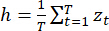   (20)

Then, the aggregated feature vector h represents the input in a compact form and serves as the classifier's input. The classification part comprises one or more dense layers, which transform the learned representation into the output space. A dense layer implements a transformation that is defined as follows:

   (21)

where o is the output (logits), b is the bias vector, and W is the weight matrix. The latter are the class scores in an unnormalized form. To incorporate nonlinearity into the model, activation functions such as ReLU are often used. Finally, a softmax activation function is applied to the logits to obtain a probability for each class:

   (22)

where C represents the number of classes, (C = 2; normal and abnormal). The class prediction will be based on the maximum probability value. During training, the optimal values of the model’s parameters are obtained by minimizing the cross-entropy loss between the actual and predicted labels, thereby achieving accurate classification of machine states. In summary, the classification layer serves an essential function in transforming the extracted temporal features using the Transformer architecture into practical decisions. Through proper discrimination between healthy and faulty machine states, anomaly detection and intelligent decision-making become possible within the Industry 5.0 paradigm.

Figure 5 shows how the classification layer works, which comes after the transformer Encoder. The process starts with the encoded sequence output, in which each vector contains temporal information learned from the input. These vectors are combined into a single vector, known as the global feature vector. The next step is to pass the global feature vector through several dense neural network layers. In each dense layer, matrix multiplication operations are performed to create linear combinations of the inputs. After that, a non-linear activation function, such as ReLU, can be applied to increase the flexibility in learning decision boundaries. At the end of the last dense layer, there are logit scores for each class. These logit scores can be used on the Softmax function to calculate probability scores for each class. These probability scores are used to determine whether the input belongs to Class 0 (Normal) or Class 1 (Abnormal).

Explainability using SHAP

After the model classifies input signals, predictions are generated based on whether the machine operates normally or abnormally. Nonetheless, within the Industry 5.0 environment, it is not enough to produce predictions; the system must also provide transparency and explainability to support human decision-making. The following framework uses SHAP, a game-theory-based model that quantifies the importance of each feature in determining the prediction. In doing so, SHAP assigns weights to features, allowing one to evaluate the relative importance of different sections of the spectrogram input to the overall prediction.

The mathematical formulation of SHAP is based on a decomposition of the model f(x):

   (23)

where ∅₀ is the baseline value (mean model output), ∅_i is the effect of the i-th feature, and M is the number of input features. For the purpose of this study, the features are the time-frequency bins from the spectrogram. SHAP values are positive if they contribute to the probability of the abnormal state and negative otherwise. This formulation guarantees a unique, locally consistent explanation for each prediction. The SHAP method can be applied to a trained CNN-transformer model to provide an explanation based on feature importance. The visual representation will show the most important time-frequency bins in the spectrogram that affect the decision-making process. For instance, abnormal behavior of the equipment may result in certain high-energy frequency bands that the SHAP framework identifies as important contributors to the decision process.

In addition, SHAP can foster cooperation between people and machines in a cyber-physical setting. This is because the predictions can be explained using intuitive visuals, allowing the operators and decision-making systems to verify predictions, analyze the problem, and take appropriate steps. This not only increases trust but also makes AI-based manufacturing processes reliable and accountable. By integrating deep learning algorithms that meet current performance standards with SHAP, which provides explainability, the proposed architecture fulfills the requirements of Industry 5.0.

Algorithm 2: SHAP-based Explainability for Model Prediction

Input: Trained model f(x), input spectrogram S

Output: SHAP values  and explanation map

Step 1: Input spectrogram S into a trained model

Step 2: Compute prediction: y = f(S)

Step 3: Initialize a deep learning-oriented SHAP explainer

Step 4: Compute SHAP values:

Step 5: For each feature i in S:

Calculate contribution 

Step 6: Generate explanation map:

Highlight regions with high 

Step 7: Visualize feature importance (heatmap)

Step 8: Return SHAP values and explanation map

The SHAP-based explainability algorithm starts by obtaining a preprocessed spectrogram image as input and feeding it into the trained CNN-transformer architecture to make predictions (e.g., normal or abnormal machine condition). After making predictions using the trained architecture, the SHAP method is used to interpret the model. In particular, the SHAP values (ϕ) are computed for each input feature to find out which time-frequency components of the input contribute most to the prediction. To calculate these values, the model outputs for inputs with and without certain features must be compared.

After calculating the SHAP values for each feature, its influence on the prediction can be evaluated by the sign and magnitude of the SHAP value. For example, features with higher SHAP values are more likely to influence the outcome, and a positive or negative sign indicates that the feature pushes the prediction toward the normal/abnormal class, respectively. Based on the results, an explanation map can be made in the form of a heatmap.

Lastly, the algorithm outputs both the SHAP values and the visualizations, providing insight into how humans can analyze the model's decision. The technique makes the process more transparent and allows humans to engage in decision-making, thus ensuring that both the algorithm's predictions and its reliability are achieved in the AI-driven industry. Representative test samples were selected from accurately diagnosed anomalous instances across various machine types to improve the reliability of the explainability analysis. While global SHAP feature-importance analysis was performed by aggregating SHAP values across the test dataset to identify consistently influential time-frequency locations, local SHAP explanations were generated for these representative cases. Without requiring expert annotation, this integrated local and global analysis offers a reliable interpretation of the model predictions.

Edge-enabled CPS Integration

This proposed solution is used within the edge-enabled CPS, which aims to achieve efficiency, sustainability, and real-time industrial operations. Once the model has been trained, the CNN-transformer will be deployed via an edge computing approach. The edge computing layer in question is near the industrial Internet of Things (IIoT) devices, including the sensors and machinery. Rather than transmitting all collected data to the cloud, the edge device performs inference on the incoming acoustic signal without first transferring it there. Therefore, the system can detect machinery abnormalities almost instantly and take the necessary steps before the situation deteriorates further. Another advantage of this edge-enabled approach is improved latency and efficiency since data is analyzed near the point of generation. In other words, unlike in the cloud approach, where inference time T_inf

   (24)

The latency, in general, will be considerably reduced through a decrease in T_{communication}. Another benefit is reduced bandwidth consumption and power expended when transmitting data continuously. This system is therefore scalable and sustainable for large industrial plants with numerous connected devices. In addition, the CPS enables interaction with the physical layer (machines), the AI (computational layer), and the human layer.

Human-in-the-loop collaboration

A key component of the suggested Industry 5.0 CPS, which includes human operators actively involved in the decision-making process alongside AI models, is human-in-the-loop collaboration. Namely, according to the designed framework, the system does not become an autonomous black box but instead allows operators to interact with it and observe explainable prediction results in the form of SHAP explanations. The predictions in question refer to the outcomes (normal/abnormal), accompanied by visualizations of parts of the spectrograms used to make them.

Such an interaction helps operators better understand exactly how the prediction is formed and which factors contribute to it. Human involvement implies verifying the system's results and allowing operators to override them when necessary, based on their professional judgment. Collaboration with human operators makes the system more trustworthy, efficient, safe, and reliable, helping prevent errors.

결과

제시된 설명 가능한 AI(Explainable AI) 통합 사이버-물리 협업 시스템은 정상 및 비정상 기계 상태가 모두 포함된 MIMII 데이터셋의 약 12,000개 오디오 녹음 파일을 통해 실험적으로 테스트되었습니다. 훈련 데이터셋은 약 9,600개의 데이터 레코드로 구성되었으며, 테스트 데이터셋에는 약 2,400개의 오디오 샘플이 포함되었습니다. 연구 결과에 따르면, 제안된 CNN-transformer 모델은 테스트 데이터셋에서 98.5%의 분류 정확도를 달성하였으며(0.97–0.98), 이는 Table 3의 결과, 혼동 행렬 및 통계적 안정성 분석과 연관됩니다. transformer 인코더를 통합함으로써 아키텍처의 시계열 모델링 능력이 향상되었으며, CNN은 입력 스펙트로그램에서 판별 가능한 공간적 특징을 추출합니다.

분류 성능 외에도 다른 시스템 관련 특성들을 평가했습니다. 첫째, 엣지 기반 구현의 추론 지연 시간은 20 ms를 초과하지 않아 실시간 이상 징후 탐지가 가능했습니다. 둘째, 제시된 시스템은 통신 요구 사항을 줄임으로써 에너지 효율을 개선하는 데 도움이 되었습니다. 마지막으로, 제안된 설명 가능한 AI(Explainable AI) 프레임워크는 SHAP 해석력을 제공하여 도메인 전문가의 관점에서 모델을 더 쉽게 분석할 수 있게 합니다. MIMII 데이터는 윈도우 크기 1024, 홉 크기 512, 고속 푸리에 변환 FFT 크기 1024를 사용하는 단시간 푸리에 변환(STFT)을 통해 스펙트로그램으로 변환되었습니다. 결과로 얻은 로그 멜-스펙트로그램은 224 × 224 픽셀로 크기를 조정하고 z-score 정규화를 수행했습니다. 학습된 모델의 강건성을 높이기 위해 시간 마스킹, 주파수 마스킹 및 가우시안 노이즈 추가를 포함한 데이터 증강 방법을 사용했습니다. CNN 아키텍처는 각각 32, 64, 128, 256개의 필터를 갖는 4개의 합성곱 층으로 구성되었으며, 배치 정규화, ReLU 및 맥스 풀링 층을 포함했습니다. 추출된 특징 맵은 시퀀스로 변환되어 트랜스포머 인코더의 입력으로 사용되었으며, 이 인코더는 4개의 인코더 층, 8개의 어텐션 헤드, 256차원 임베딩 및 1024차원 피드포워드 차원으로 구성되었습니다. 과적합을 최소화하기 위해 0.3의 드롭아웃 확률을 적용했습니다. 학습에는 학습률 0.0001과 가중치 감쇠 1 x 10⁻⁵의 Adam 옵티마이저가 사용되었습니다. 학습 시 에포크 수와 배치 크기는 각각 100과 32였습니다. 실험 재현성을 유지하기 위해 랜덤 시드는 42로 설정되었습니다. 결과의 통계적 유효성을 검증하기 위해 다음 방법들이 사용되었습니다. 모든 실험은 서로 다른 랜덤 시드와 데이터 셔플링을 통해 10회 독립적으로 수행되었습니다. 정확도(Accuracy), 정밀도(Precision), 재현율(Recall), F1-스코어(F1-score), ROC 곡선 아래 면적(ROC-AUC) 및 정밀도-재현율 곡선 아래 면적(PR-AUC)의 평균값과 표준 편차를 계산했습니다. 또한, 성능 불확실성을 추정하기 위해 95% 신뢰 구간을 계산했습니다. 마지막으로, 본 연구의 CNN-트랜스포머 방식과 가장 성능이 좋은 베이스라인 모델의 결과를 비교하여 대응 표본 t-검정을 수행했습니다. 조기 종료 방법은 patience 파라미터를 10 에포크로 설정하여 적용했습니다. 표 4는 환경 설정 및 하이퍼파라미터 구성을 나타내며, 표 5는 시뮬레이션 환경의 세부 사항을 제공합니다.

본 연구의 평가 실험은 다양한 기계 작동 조건과 음향 결함 시나리오가 포함된 MIMII 데이터셋을 사용하여 수행되었습니다. 제안된 프레임워크의 결과가 모델을 검증하였으나, 다양한 산업 데이터셋과 제조 환경에 걸친 추가적인 검증이 필요합니다.

제안된 프레임워크는 실시간 추론과 설명 가능성을 지원하기 위해 멀티코어 프로세서, 16 GB 시스템 메모리 및 그래픽 처리 장치(GPU) 기반의 엣지 가속기가 장착된 엣지 컴퓨팅 플랫폼에서 구현되었습니다. 산업용 음향 센서는 IIoT 통신 계층을 통해 오디오 스트림을 엣지 게이트웨이로 전송했습니다. 엣지 노드는 스펙트로그램 생성, 이상 징후 추론 및 SHAP 설명 생성과 같은 작업을 수행하는 데 사용되었으며, 클라우드 서버는 장기 데이터를 저장하고 모델을 업데이트하는 데 사용되었습니다. 이러한 구성은 필요한 통신량을 줄일 뿐만 아니라, 사이버 물리 시스템 내의 센싱 장치, AI 모듈 및 인간 작업자 간의 실시간 상호 작용을 가능하게 합니다.

위에서 소개한 CNN-transformer 방식은 서포트 벡터 머신(SVM) 및 랜덤 포레스트와 같은 전통적인 ML 모델, transformer가 없는 CNN 모델, 그리고 long short-term memory(LSTM) 기반 방식 등 여러 기존 방법들과 비교되었습니다. 전통적인 ML 모델은 데이터의 공간적 및 시간적 상관관계를 처리하는 능력이 부족하여 만족스러운 결과를 얻지 못한 반면, CNN 모델은 공간적 특징을 효율적으로 처리할 수 있고, LSTM 모델은 음향 신호의 시간적 측면을 처리할 수 있습니다. 그럼에도 불구하고, 전자(CNN)는 후자(LSTM)에 비해 계산 비용과 병렬 처리 능력 면에서 열세에 있습니다.

제안된 CNN-transformer 모델과 베이스라인 모델 간의 공정한 비교를 위해, 전자는 동일한 MIMII 데이터셋 분할(훈련 80%, 테스트 20%), 전처리 단계, 스펙트로그램 생성 과정 및 평가 지표를 사용하여 훈련 및 평가되었습니다. SVM 방법에서는 C = 10 및 γ = 0.01인 방사 기저 함수(RBF) 커널을 사용하였습니다. 랜덤 포레스트 방법은 최대 트리 깊이 20의 트리 200개를 포함하였습니다. CNN의 경우, Transformer 모듈 없이 4개의 컨볼루션 층(필터 32, 64, 128, 256개)과 그 뒤를 잇는 완전 연결 층으로 구성되었습니다. 마지막으로 LSTM 방법의 경우, 128개의 은닉 유닛과 0.3의 드롭아웃 비율을 가진 두 개의 적층형 LSTM 층을 사용하였습니다.

반면에, CNN-transformer 프레임워크를 사용하면 음향 신호의 공간적 및 시간적 능력을 모두 효율적으로 활용하여 최적의 결과를 얻을 수 있습니다. 또한, 엣지 컴퓨팅을 사용하면 컴퓨팅 비용을 절감하고 지연 시간을 개선하며 에너지를 절약할 수 있습니다. 이에 더해, SHAP을 통해 구현된 예측의 설명 가능성은 제안된 방법이 기존 기술과 차별화되는 또 다른 장점으로 간주될 수 있습니다.

Vision Transformer (ViT), Audio Spectrogram Transformer (AST), Conformer 및 자기지도 학습 기반 모델과 같은 음향 이상 탐지를 위한 새로운 모델 개발의 최근 성과에도 불구하고, 본 연구에서는 이러한 아키텍처들의 실험적 비교를 수행하지 않았습니다. 향후에는 이러한 모델들을 제안된 프레임워크를 평가하기 위한 벤치마크로 사용할 계획입니다.

제안된 모델의 성능을 평가하기 위해 정확도(accuracy), 정밀도(precision), 재현율(recall) 및 F1-score를 포함한 지표들이 사용됩니다. 정확도가 예측의 전반적인 정답률을 평가하는 반면, 정밀도는 전체 정탐(true positive) 및 오탐(false positive) 수 대비 정탐의 비율을 측정합니다. 재현율은 특정 시스템의 이상 징후를 예측하는 모델의 능력을 추정하여 제공합니다. 결함을 예측하지 못하는 것은 시스템 붕괴로 이어질 수 있기 때문에 이는 매우 중요합니다. 이러한 지표들의 수학적 계산 방법은 다음과 같습니다.

   (25)

   (26)

   (27)

   (28)

이 외에도, 엣지 컴퓨팅 기반의 제안된 CPS 모델의 실제 성능을 평가할 때 지연 시간, 에너지 활용도, 확장성과 같은 시스템 성능 관련 추가 지표들이 고려됩니다.

표준 성능 측정 기법 외에도, 특히 실제 환경의 불균형 및 스트리밍 데이터 사례 연구에 대한 적용 가능성을 고려할 때, 제안된 솔루션을 보다 종합적인 관점에서 평가하는 데 도움이 되는 여러 다른 측정 지표들이 있습니다. 예를 들어, 서로 다른 임계값을 기반으로 두 그룹을 구별하는 알고리즘의 능력은 ROC 곡선 아래 면적(ROC-AUC)으로 측정됩니다. 강건성과 분리 능력이 우수하다면 ROC-AUC 값은 높게 나타나야 합니다. 또한, 이상 클래스가 드물게 나타나는 이상 탐지 사례 연구에서는 정밀도-재현율 곡선 아래 면적(PR-AUC) 지표가 중요합니다.

고려해야 할 중요한 척도는 매튜스 상관계수(Matthews Correlation Coefficient, MCC)입니다. 이는 혼동 행렬의 네 가지 항목을 모두 고려하므로, 클래스 불균형이 존재하는 경우에도 정확한 평가를 제공합니다. 이 척도는 다음과 같이 계산됩니다:

   (29)

MCC 값의 범위는 -1에서 +1까지이며, +1은 완벽한 예측을 나타냅니다. 적용 가능한 또 다른 지표로는 특이도(True Negative Rate)가 있으며, 이는 위양성 예측이 있는지 평가하는 산업적 응용 분야에서 유용할 수 있습니다:

    (30)

혼동 행렬과 성능 지표 간의 불일치가 없음을 보장하기 위해, 모든 평가 기준은 최종 테스트 데이터셋을 기반으로 계산되었습니다. 이후의 식에서는 진양성(TP), 진음성(TN), 위양성(FP) 및 위음성(FN) 표기법이 사용됩니다. 정확도, 정밀도, 재현율, 특이도, F1-score 및 MCC는 식 (25)–(30)을 기반으로 산출되었습니다. 또한, 독립적인 임계값 평가를 통해 CNN-transformer 모델의 확률 출력값으로부터 ROC-AUC와 PR-AUC를 계산하였습니다.

시스템 수준에서 고려해야 할 핵심 지표에는 지연 시간, 처리량 및 계산 비용이 포함됩니다. 지연 시간은 예측을 수행하는 데 필요한 시간입니다. 처리량은 초당 처리되는 데이터 샘플의 양입니다. 에너지 효율성을 나타내는 계산 비용은 계산 효율성을 보장하는 데 중요합니다. 또한, 모델을 평가할 때 SHAP 일관성 및 특성 중요도의 안정성과 같은 설명 가능성 지표도 고려될 수 있습니다.

MIMII 데이터셋에 대한 Table 3의 결과로부터 제안된 CNN-transformer 모델이 다른 모든 머신러닝 및 딥러닝 방법보다 성능이 뛰어나다는 것이 분명히 드러납니다. SVM과 랜덤 포레스트 모델의 성능은 각각 88.6%와 91.2%의 정확도를 보이며 수용 가능한 수준이나 제한적입니다. 이는 해당 모델들이 음향 신호에서 복잡한 시간적 및 공간적 특징을 추출하지 못하기 때문으로 설명될 수 있습니다. 반면, LSTM은 시계열 데이터를 모델링함으로써 94.5%의 정확도를 달성하여 SVM과 랜덤 포레스트보다 우수한 성능을 보였습니다. 그러나 제안된 CNN-transformer 방식은 정확도(98.5%), 정밀도(98.06%), 재현율(99.02%) 및 F1-score(98.54%)가 향상되어 가장 우수한 성능을 나타냅니다. 따라서 제안된 알고리즘은 기계의 정상 및 비정상 상태를 정확하게 분류할 수 있습니다. 향상된 특이도(97.96%)는 산업 현장에서 매우 중요한 요소인 위양성(false positives)을 줄이는 데 이 방식이 효과적임을 보여줍니다. CNN-transformer의 이러한 성능은 CNN이 판별 특징을 추출하고 Transformer가 긴 시퀀스의 시간적 관계를 포착하는 두 구조의 결합으로 설명될 수 있습니다.

그림 6의 ROC 곡선은 MIMII 데이터셋에 대한 분류 능력과 관련하여 SVM, 랜덤 포레스트, LSTM 및 제안된 CNN-transformer 접근 방식의 비교 성능을 보여줍니다. 그림 6에서 보듯, 제안된 CNN-transformer에서 0.994라는 가장 높은 곡선 아래 면적(AUC)이 관찰되었습니다. 이는 제안된 방법이 정상 및 비정상 범주를 구별하는 데 있어 더 우수한 판별 성능을 제공함을 분명히 보여줍니다. 반면, LSTM은 제안된 CNN-transformer 방식보다 약간 낮은 결과를 보이며, AUC는 약 0.97입니다. 랜덤 포레스트와 SVM은 각각 약 0.958 및 0.913으로 상대적으로 낮은 AUC를 나타냅니다. 이는 두 방식 모두 주어진 데이터로부터 복잡한 음향 패턴을 학습하는 능력이 부족하기 때문입니다.

이상치 탐지에서는 이상 샘플의 수가 적기 때문에 정밀도-재현율(PR) 곡선이 더 나은 분석을 제공합니다. 그림 7에 나타난 바와 같이, PR 곡선에서 CNN-transformer 모델은 약 0.97–0.98의 가장 높은 평균 정밀도(AP)를 달성하여, 오경보를 줄이면서 이상 사례를 탐지하는 능력이 우수함을 시사합니다. 반대로, LSTM 분류기는 0.92에서 0.94 범위의 AP로 2위를 기록했습니다. 한편, 랜덤 포레스트와 SVM 분류기는 각각 0.88과 0.84의 AP로 3위와 4위에 올랐습니다. 제안된 하이브리드 분류기는 모든 재현율 수준에서 더 높은 정확도를 달성했으며, 이는 높은 정밀도와 낮은 오경보율을 모두 요구하는 실제 산업 응용 분야에서 매우 중요합니다.

CNN-transformer 모델을 Table 6에 제시된 고급 성능 지표를 사용하여 MIMII 데이터셋의 기존 모델들과 비교하였습니다. ROC-AUC 값은 다양한 임계값에서 두 클래스를 구분하는 모델의 판별 능력을 나타냅니다. SVM과 랜덤 포레스트 분류기는 각각 0.913과 0.958의 ROC-AUC 값을 기록했으며, LSTM 모델은 0.970, CNN은 0.98을 달성했습니다. 제안된 CNN-transformer 프레임워크는 0.994로 가장 높은 ROC-AUC를 기록하여, 정상 및 비정상 기계 상태 간의 우수한 판별 능력을 입증했습니다. 마찬가지로, PR-AUC 값은 제안된 모델이 이상 탐지에서 필수적인 요소인 클래스 불균형 문제를 효과적으로 처리할 수 있음을 보여줍니다. 제안된 CNN-transformer는 0.982로 가장 높은 PR-AUC(평균 정밀도)를 달성했으며, CNN(0.950), LSTM(0.912), 랜덤 포레스트(0.891), SVM(0.765)이 그 뒤를 이어 산업용 음향 이상 탐지에서 우수한 정밀도-재현율 성능을 나타냈습니다. 또한, 모델 성능의 균형을 측정하는 매튜스 상관 계수(MCC)는 제안된 모델에서 0.97이라는 비교적 높은 값으로 나타났습니다. 반면, SVM(0.73) 및 랜덤 포레스트(0.78)와 같은 기존 방법들은 더 낮은 예측 정확도를 보였습니다.

제시된 접근 방식의 안정성을 테스트하기 위해, 서로 다른 초기화 시드와 데이터 셔플링 체계로 동일한 실험을 10회 수행하였습니다. CNN-transformer 아키텍처에 대한 Table 7의 결과는 다음과 같았습니다: accuracy = 98.50% ± 0.19%, precision = 98.06% ± 0.23%, recall = 99.02% ± 0.22%, F1-score = 98.54% ± 0.24%. 상대적으로 작은 표준 편차는 모델의 안정성을 나타냅니다. 모든 평가 지표에 대해 95% 신뢰 구간을 계산하였습니다. accuracy 지표의 신뢰 구간은 [98.1%, 98.9%]로 결정되었으며, 이는 모델이 일관되게 우수한 성능을 보임을 나타냅니다. ROC-AUC, PR-AUC 및 MCC에 대해서도 좁은 신뢰 구간이 확인되었습니다. 제안된 CNN-transformer 모델과 가장 성능이 좋은 베이스라인 모델(LSTM)을 비교한 paired t-test 결과 p value < 0.05로 나타났으며, 이는 관찰된 성능 향상이 우연에 의한 것이 아니라 통계적으로 유의미함을 나타냅니다.

제안된 CNN-transformer 아키텍처의 견고성을 테스트하기 위해, 그림 8에 나타낸 바와 같이 서로 다른 무작위 초기화 시드와 셔플링 구성을 사용하여 실험을 10회 반복하였습니다. 모델을 통해 얻은 평균 정확도, 정밀도, 재현율 및 F1-score는 각각 98.50% ± 0.19%, 98.06% ± 0.23%, 99.02% ± 0.22%, 98.54% ± 0.24%였습니다. 박스 플롯 분석 결과, 모델의 성능 지표에서 변동이 매우 적게 나타나 안정성과 견고함을 확인하였습니다. 따라서 제안된 접근 방식은 여러 차례의 실험에서 유의미한 변동 없이 높은 안정성을 보였으며, 이는 모델의 우수한 일반화 능력을 나타냅니다.

또한, 실험의 여러 차례 실행 결과물을 바탕으로 통계적 검정을 수행하였습니다. 모든 평가 지표에서 표준 편차가 작게 나타난 것은 무작위성이나 학습의 변화에 대한 민감도가 낮음을 시사합니다. 이는 제안된 CNN-transformer 모델이 실제 사이버 물리 제조 시스템에서 안정적이고 일관된 성능을 제공할 수 있음을 확인시켜 줍니다.

SHAP 히트맵은 기계 상태가 정상인지 비정상인지 예측하는 데 있어 스펙트로그램의 시간-주파수 영역이 갖는 중요도를 보여줍니다. SHAP 값은 최종 예측에 대한 각 예측 변수의 기여도를 나타냅니다.

그림 9A에 표시된 SHAP 값 히트맵에서 양수 SHAP 값(예: +0.6에서 +1.2 사이)은 이상 상태에 대한 기여도를 나타내며, 음수 SHAP 값(즉, −0.3에서 −0.8 사이)은 정상 범주에 대한 기여도를 나타냅니다. 가장 강한 SHAP 점수는 시간 프레임 50–100의 중간 주파수 범위(40–80 주파수 빈)에서 발견되었습니다. 이 영역들은 음향 측정에서 임계 결함 신호가 검출되는 핵심 영역입니다. 또한, 저주파 대역(20개 미만의 빈)은 SHAP 점수가 거의 0(−0.1에서 +0.1)으로 나타나, 모델의 의사결정에 미치는 영향이 무시할 수 있는 수준임을 보여줍니다. 이는 모델이 결함 예측과 무관한 배경 소음을 무시한다는 것을 나타냅니다. 특정 시간 대역 내에서 높은 SHAP 점수가 시간적 일관성을 보이는 것은 음향 신호의 장거리 의존성을 포착하는 Transformer 모듈의 능력을 강조합니다. 요약하면, SHAP 히트맵은 CNN-transformer 모델이 변별력이 높은 고유한 시간-주파수 대역에 집중한다는 것을 명확히 보여줍니다. 이는 모델의 해석 가능성을 높이며 작업자가 시각적으로 결함을 감지하는 데 도움을 줍니다.

SHAP 방법은 오직 해석 가능성을 위한 기술로만 사용되며, CNN-transformer 모델의 학습 과정에는 포함되지 않음을 보여줍니다. 분류 정확도는 오직 CNN 및 Transformer 구성 요소에 의해 학습된 파라미터에 의해서만 결정됩니다. SHAP은 모델 추론 단계 이후에 사용되어, 예측을 정상 또는 비정상 범주로 유도하는 가장 영향력 있는 시간-주파수 윈도우를 식별함으로써 예측 결과를 해석합니다. 따라서 SHAP은 분류 정확도에 영향을 주지 않으면서 인간의 투명성과 이해도를 높여줍니다. 제안된 프레임워크에서 제공하는 SHAP 값은 명확한 시각화를 가능하게 하여, 유지보수 작업자가 검출된 영역을 실제 기계 동작 및 유지보수 기록과 비교함으로써 모델의 예측을 검증하는 데 도움을 줍니다. 결과적으로 예측 유지보수 활동 중 인간과 기계가 더 쉽게 협업할 수 있게 됩니다.

설명 가능성 수준을 평가하기 위해 그림 9B에 나타낸 바와 같이 특성 중요도에 대한 전역 SHAP 분석을 수행하였다. 결과에 따르면 일부 중간 주파수 성분이 이상 탐지에서 중요한 역할을 하는 것으로 나타났다. 또한, 그림 9C에 제시된 사례 연구는 SHAP이 이상 기계 스펙트로그램에서 결함 관련 영역을 정확하게 식별함을 보여준다. 본 연구에서는 MIMII 데이터셋의 펌프 및 밸브 이상 데이터 샘플을 활용하여 정성적 사례 연구를 진행하였다. 결함이 있는 펌프의 경우, SHAP은 공동 현상(cavitation) 및 마모와 관련된 2–4 kHz 주파수 범위를 식별하였다. 결함이 있는 밸브의 경우, 누설을 나타내는 반복적인 고조파 신호 영역에서 SHAP 활성화가 지배적으로 나타났다. 대표적인 테스트 샘플 전반에 걸쳐, SHAP 시각화는 이상 기계 상태와 관련된 판별적 시간-주파수 영역을 신뢰성 있게 식별하였다. 각 예측에 가장 크게 기여하는 스펙트럼 영역을 강조함으로써, 이러한 설명은 모델이 어떻게 결정을 내리는지에 대한 통찰을 제공한다. 유지보수 전문가에 의한 공식적인 검증은 본 연구의 범위를 벗어났으므로, SHAP 분석은 전문가가 검증한 결함 확인이 아닌 모델 동작을 이해하기 위한 해석 도구로 제공된다.

혼동 행렬(confusion matrix)은 그림 10에 제시된 MIMII 데이터셋에 대해 제안된 CNN-transformer 모델의 분류 성능이 얼마나 우수한지를 보여줍니다. 전반적으로 960개의 정상 샘플이 정상으로 정확하게 식별되었으며(진음성), 20개의 정상 샘플은 비정상으로 잘못 식별되었습니다(위양성). 또한, 전체 샘플 중 1010개의 비정상 샘플이 비정상으로 검출되었고(진양성), 10개의 비정상 샘플은 정상으로 식별되었습니다(위음성).

따라서 특히 예측 보전에서 매우 중요한 이상 샘플에 대해 높은 검출 성능을 달성하였습니다. 그림 10에서 보듯이, 미검출(False Negative) 오류는 매우 드물게(10개 샘플) 관찰되었으며, 이는 산업 전반의 안전성과 신뢰성을 보장하는 데 있어 필수적인 요소입니다. 반면, 오검출(False Positive) 오류(20개 샘플)는 약간 더 자주 발생하지만 여전히 상대적으로 낮은 수준을 유지하고 있습니다. 그림 10에 제시된 혼동 행렬(confusion matrix)은 분류기의 성능을 명확하게 시각화하기 위해 2,000개의 테스트 기록(정상 및 이상 샘플의 수가 동일함)으로 구성된 균형 잡힌 하위 집합을 사용하여 생성되었습니다. 정확도, 정밀도, 재현율, 특이도 및 F1-스코어를 포함하여 보고된 모든 평가 지표는 전체 테스트 세트(약 2,400개 기록)를 사용하여 계산되었습니다.

~에 묘사된 혼동 행렬(confusion matrix)을 고려하면 그림 10 및 ~에서 표 8 (TN = 960, FP = 20, TP = 1010, FN = 10)일 때, 다음과 같이 계산할 수 있습니다: 정확도(Accuracy) = (TP + TN) / (TP + TN + FP + FN) = 98.50%, 정밀도(Precision) = TP/(TP + FP) = 98.06%, 재현율(Recall) = TP/(TP + FN) = 99.02%, 특이도(Specificity) = TN / (TN + FP) = 97.96%, F1-스코어(F1-score) = 98.54%, 그리고 MCC = 0.97입니다. 또한, ROC-AUC 및 PR-AUC 값은 각각 0.994와 0.982였습니다. 다음에 제시된 혼동 행렬(confusion matrix)은 그림 10 시각화 목적으로만 테스트 데이터에서 균형 있게 추출한 2,000개 녹음 파일의 대표 하위 집합을 사용하여 생성되었습니다. 본 연구에서 보고된 모든 정량적 성능 지표는 전체 테스트 세트(약 2,400개 녹음 파일)를 사용하여 계산되었습니다. 전반적으로, 결과는 제안된 CNN-트랜스포머 아키텍처가 98.5%의 분류 정확도를 달성했음을 보여주며, 이는 다음의 보고된 결과와 일치합니다. 표 8 그리고 어블레이션 분석(ablation analysis)입니다.

에지 기반 구현의 효과를 검증하기 위해 추가 측정을 수행하였습니다. 표 9에 나타난 바와 같이, 제안된 모델의 평균 추론 지연 시간은 18.7 ms/sample이며, 초당 약 53개의 샘플을 처리할 수 있습니다. 추론 중 전력 소모량은 8.9 W였으며, 예측당 추정 에너지 소비량은 0.167 J/prediction으로 산출되었습니다. 표 10에서는 제안된 접근 방식의 지속 가능성 영향을 평가하기 위해 통신 오버헤드, 에너지 소비 및 리소스 사용량을 고려하였습니다. 추론 프로세스가 에지 노드에서 로컬로 수행되므로, 요약된 진단 데이터만 클라우드 환경으로 전송됩니다. 실험 결과, 기존의 클라우드 기반 CPS 시스템과 비교하여 통신량이 73% 감소한 것으로 나타났습니다. 또한, 로컬 추론을 통해 에너지 소비는 32% 감소하였으며, 통신 시간은 75 ms에서 20 ms로 단축되었습니다.

어블레이션 연구

설명 가능한 AI 기반 CPHS 아키텍처의 각 구성 요소가 미치는 영향을 평가하기 위해 MIMII 데이터셋에 대해 제거 연구(ablation research)를 수행합니다. 본 제거 연구에서는 공간적 특징을 학습하기 위한 CNN, 시간적 특징을 학습하기 위한 트랜스포머 인코더, 그리고 SHAP 설명 가능성 알고리즘 자체의 효과를 조사합니다. 제안된 모델의 몇 가지 수정 버전이 고려되었는데, 구체적으로는 (i) CNN 전용 버전, (ii) 트랜스포머 전용 버전, (iii) CNN과 트랜스포머는 결합되었으나 SHAP 알고리즘은 제외된 모델, (iv) CNN과 트랜스포머가 SHAP과 결합된 전체 제안 모델입니다. 평가를 위해 정확도(accuracy), 정밀도(precision), 재현율(recall) 및 F1-스코어(F1-score)와 같은 일반적인 지표가 사용됩니다.

이러한 어블레이션 연구 결과는 Table 11에 설명된 프레임워크의 각 요소가 갖는 중요성을 입증합니다. CNN 전용 모델은 93.8%의 정확도를 달성하여 스펙트로그램으로부터의 공간적 특징 추출이 효과적임을 보여주었으나, 음향 신호의 시간적 의존성은 캡처하지 못했습니다. 이는 Transformer 전용 모델에도 동일하게 적용되며, 해당 모델은 공간적 정보를 무시하고 시간적 특징을 추출하기 때문에 약간 더 낮은 정확도(92.6%)를 보였습니다. 마지막으로, 제안된 CNN-transformer 모델은 메인 실험 결과와 일치하게 98.5%의 정확도, 98.06%의 정밀도, 99.02%의 재현율 및 98.54%의 F1 스코어를 얻었습니다. SHAP은 모델 학습이 아닌 사후 해석(post hoc interpretation)에만 사용되므로, 분류 정확도는 학습된 CNN-transformer 모델과 동일합니다. 이후 SHAP은 특징 기여도 설명을 생성하는 데 사용됩니다. 향상된 재현율(99.02%)은 모델이 기계의 이상 상태를 감지하는 데 효과적이며, 결함 부품을 누락 없이 찾아낼 수 있음을 나타내며, 이는 예지 보전 시스템 구현에 있어 필수적입니다.

데이터 가용성:

본 연구에 사용된 Malfunctioning Industrial Machine Investigation and Inspection (MIMII) 데이터셋은 공식 Zenodo 저장소에서 공개적으로 제공됩니다. 실험은 데이터셋 저자가 제공한 공개 오디오 녹음 및 어노테이션을 사용하여 수행되었습니다. 데이터셋은 https://zenodo.org/records/3384388에서 확인할 수 있습니다. 본 연구와 함께 제공되는 구현 코드는 Zenodo 저장소 https://zenodo.org/records/21405292를 통해 공개적으로 제공됩니다. 해당 저장소에는 데이터 전처리 파이프라인, 모델 아키텍처, 학습 워크플로우, 평가 스크립트, 설정 파일 및 제안된 방법론의 이해와 독립적인 재현을 돕기 위한 지원 유틸리티를 포함하여, 제안된 프레임워크의 구현 코드가 포함되어 있습니다. MIMII 데이터셋은 구현 코드와 함께 재배포되지 않으며, 공식 저장소에서 별도로 취득해야 합니다.

그림 1: 제안된 연구의 아키텍처. 지속 가능한 제조를 위해 전처리, CNN 기반 공간 학습, 트랜스포머 기반 시계열 모델링, SHAP 설명 가능성 및 엣지 컴퓨팅을 결합한 설명 가능한 AI 기반 사이버-물리 인간 시스템의 아키텍처 설계. 이 그림의 더 큰 버전을 보려면 여기를 클릭하십시오.

그림 2: 전처리 파이프라인. 노이즈 제거, 정규화, 세그먼트 분할, STFT 변환 및 스펙트로그램 추출로 구성된 음향 신호 전처리 파이프라인. 여기에서 이 그림의 확대 버전을 확인하십시오.

그림 3: CNN을 이용한 공간 특징 추출. 컨볼루션(convolution), 활성화(activation) 및 풀링(pooling) 과정을 통해 스펙트로그램을 사용하여 CNN으로 공간 특징을 추출하는 아키텍처. 이 그림의 더 큰 버전을 보려면 여기를 클릭하십시오.

그림 4: 트랜스포머 인코더를 이용한 시간적 모델링. 스펙트로그램 시퀀스 표현을 통해 시간적 의존성과 장거리 의존성을 포착하는 트랜스포머 인코더 아키텍처. 이 그림의 더 큰 버전을 보려면 여기를 클릭하십시오.

그림 5: 분류층 인코딩된 시계열 특징을 기계 상태 예측을 위한 확률 값으로 매핑하는 분류기 층입니다. 이 그림의 더 큰 버전을 보시려면 여기를 클릭하십시오.

그림 6: ROC 곡선 결과. MIMII 데이터셋에 대한 SVM, random forest, LSTM, CNN 및 제안된 CNN-transformer 알고리즘의 ROC 곡선 비교. 이 그림의 더 큰 버전을 보려면 여기를 클릭하십시오.

그림 7: 정밀도-재현율 곡선 결과. 다양한 머신러닝 및 딥러닝 방법의 이상 탐지 효율을 나타내는 정밀도-재현율 곡선 비교. 이 그림의 더 큰 버전을 보려면 여기를 클릭하십시오.

그림 8: 다회 반복 실행 성능 안정성 분석. 제안된 CNN-transformer 아키텍처를 사용하여 수행한 10번의 독립적인 실험에서 얻은 Accuracy, Precision, Recall 및 F1-score 결과의 성능 안정성을 보여주는 박스 플롯. 작은 변동폭은 모델의 안정성과 강건성을 나타낸다. 여기를 클릭하여 이 그림의 확대 버전을 확인하십시오.

그림 9: 제안된 이상 탐지 프레임워크의 SHAP 기반 설명 가능성 분석. (A) SHAP 기반 설명 가능성 분석. 이상 행동 식별을 유도하는 가장 관련성 높은 시간-주파수 영역을 보여주는 SHAP 방법 기반의 히트맵. (B) 가장 영향력 있는 특성을 식별하기 위한 전역 SHAP 접근 방식을 이용한 특성 중요도 분석. (C) 비정상 기계에 대한 SHAP 설명 가능성 시각화. 이 그림의 더 큰 버전을 보시려면 여기를 클릭하십시오.

그림 10: MIMII 데이터셋에 대한 혼동 행렬. 혼동 행렬은 제안된 CNN-transformer 알고리즘의 분류 성능을 나타냅니다. 여기를 클릭하여 이 그림의 더 큰 버전을 확인하십시오.

매개변수	설명
데이터셋 이름	MIMII (Malfunctioning Industrial Machine Investigation and Inspection) 데이터셋
기계 유형	밸브, 펌프, 팬, 슬라이드 레일
사용된 총 샘플 수	약 12,000개의 오디오 녹음 파일
클래스	정상, 비정상
샘플링 레이트	16 kHz
샘플당 지속 시간	10초
오디오 형식	WAV
특징 표현	STFT 기반 스펙트로그램 이미지
전처리 단계	노이즈 필터링, 정규화, 세그멘테이션, STFT 변환
레이블 할당	MIMII 주석에 따라 정상 녹음은 클래스 0, 비정상 녹음은 클래스 1로 레이블링
훈련-테스트 분할	80% 훈련 (≈9,600개 샘플), 20% 테스트 (≈2,400개 샘플)
데이터 분할 전략	데이터 누수를 방지하기 위해 세그멘테이션 전에 오디오 파일 수준의 분할 수행
산업 노이즈 조건	MIMII 녹음에 포함된 실제 산업 음향 환경
응용 분야	예측 보전 및 기계 이상 탐지
대상 Industry 5.0 목표	설명 가능하고 인간 중심적이며 지속 가능한 결함 탐지

표 1: 데이터셋 설명. 기계 유형, 샘플링 분포, 신호 특성, 특징 표현 및 응용 측면과 관련한 MIMII 데이터셋에 대한 설명.

장비 유형	기기 ID	정상 기록	이상 기록	SNR 조건 (dB)	실험적 분할
팬	ID00–ID06	8,400	1,600	−12에서 −9까지	80% 훈련 / 20% 테스트
기어박스	ID00–ID06	7,124	1,147	−17 ~ −15	80% 훈련 / 20% 테스트
펌프	ID00–ID06	7,200	1,800	−18 ~ −9	80% 훈련 / 20% 테스트
슬라이드 레일	ID00–ID05	7,000	1,800	−14 ~ −12	80% 훈련 / 20% 테스트
밸브	ID00–ID05	7,000	1,800	−12에서 −9까지	80% 훈련 / 20% 테스트

표 2: 본 연구에 사용된 MIMII 데이터셋에 대한 설명. 산업용 기계 유형, 기계 ID, 정상 및 이상 기록 횟수, SNR 조건, 그리고 지도 학습 기반 이진 분류에 사용된 훈련/테스트 분할.

모델	정확도 (%)	정밀도 (%)	재현율 (%)	F1-스코어 (%)	특이도 (%)
SVM	88.6	86.9	85.4	86.1	90.2
Random Forest (RF)	91.2	89.8	88.5	89.1	92.6
LSTM	94.5	93.2	92.8	93	95.1
CNN	96.3	95.4	94.9	95.1	96.8
CNN–Transformer (제안됨)	98.5	98.06	99.02	98.54	97.96

표 3: MIMII 데이터셋에 대한 분류 결과. 정확도, 정밀도, 재현율, F1 스코어 및 특이도를 이용한 머신러닝 및 딥러닝 분류기의 성능 비교.

매개변수	값
데이터셋	MIMII 데이터셋
총 시료 수	~12,000
훈련-테스트 분할	80% / 20%
입력 유형	스펙트로그램 이미지
CNN 층	3~5개 합성곱 층
트랜스포머 층	2~4개 인코더 층
배치 크기	32
학습률	0.001
최적화 알고리즘	아담
에포크(Epochs)	100
하드웨어	엣지 디바이스 + GPU (학습용)
STFT 윈도우 길이	1024
홉 크기	512
FFT 크기	1024
스펙트로그램 해상도	224 × 224
정규화	Z-점수
데이터 증강	시간 마스킹, 주파수 마스킹, 가우시안 노이즈
CNN 층	4
CNN 필터	32, 64, 128, 256
트랜스포머 층	4
어텐션 헤드	8
임베딩 차원	256
피드포워드 차원	1024
드롭아웃	0.3
난수 시드	42
조기 종료 인내심(Early Stopping Patience)	10

표 4: 환경 설정 및 하이퍼파라미터 구성. 제안된 CNN-transformer 아키텍처를 구현하는 데 사용된 훈련 및 실험 파라미터.

구성 요소	사양서
프로그래밍 언어	파이썬
프레임워크	TensorFlow / PyTorch
프로세서	Intel i7 / Ryzen 7
그래픽 처리 장치(GPU)	NVIDIA GTX 1660 / RTX 시리즈
엣지 디바이스	Raspberry Pi / NVIDIA Jetson
시각화	Matplotlib, SHAP
엣지 디바이스	NVIDIA Jetson Xavier NX
중앙 처리 장치	6코어 ARM v8.2
랜덤 액세스 메모리(RAM)	16 GB
운영체제	Ubuntu 20.04
딥러닝 프레임워크	TensorFlow/PyTorch
데이터셋 크기	12,000개의 MIMII 샘플
연결성	이더넷/와이파이
모델 파라미터	840만
모델 크기	32.7 MB
프레임워크	PyTorch + TensorRT
배치 크기	1
양자화	FP16
가지치기	아니요
평균 잠복기	17.8 ms
중앙값 잠복기	17.2 ms
95 백분위수 지연 시간	19.6 ms
처리량	56 샘플/초
메모리 사용량	1.4 GB
전력 소비량	11.3 W

표 5: 시뮬레이션 환경.제안된 모델을 학습, 배포 및 평가하는 데 사용된 하드웨어와 소프트웨어입니다.

모델	ROC-AUC (수신자 조작 특성-곡선 아래 면적)	PR-AUC	정전용량성 결합(MCC)
서포트 벡터 머신(SVM)	0.913	0.765	0.73
랜덤 포레스트 (Random Forest, RF)	0.958	0.891	0.78
장단기 메모리(LSTM)	0.97	0.912	0.86
합성곱 신경망(CNN)	0.98	0.95	0.9
CNN–Transformer (제안 방식)	0.994	0.982	0.97

표 6: ROC-AUC, PR-AUC 및 MCC의 실험 결과 비교. ROC-AUC, PR-AUC 및 Matthews 상관 계수 측정값에 기반한 다양한 모델 간의 비교.

평가 지표	평균 (%) + 표준편차(%)	95% 신뢰 구간
정확도(Accuracy)	98.50 ± 0.19	[98.1, 98.9]
정밀도(Precision)	98.06 ± 0.23	[98.0, 98.2]
재현율(Recall)	99.22 ± 0.22	[98.8, 99.4]
F1-score	98.54 ± 0.24	[98.1, 98.9]
ROC-AUC	0.984	0.004
PR-AUC	0.982	0.005
MCC	0.97	0.007

표 7: 다회 실행 통계 분석 결과. 다양한 성능 측정 지표에 대한 평균, 표준 편차, 95% 신뢰 구간 및 유의성을 포함하여, 제안된 CNN-transformer 아키텍처의 10회 실험에 걸친 강건성 통계.

측정 지표	값
정확도	98.50%
정밀도	98.06%
재현율	99.02%
특이도	97.96%
F1-스코어	98.54%
MCC	0.97
ROC-AUC	0.994
PR-AUC	0.982

표 8: 혼동 행렬의 최종 테스트 세트. 제안된 아키텍처에 대한 테스트 세트 혼동 행렬로, 평가 지표의 도출 근거가 된 기계의 정상 및 비정상 상태 분류 결과가 나타나 있다.

측정 지표	클라우드 배포	엣지 배포
추론 지연 시간(ms)	85.6	18.7
처리량 (샘플/초)	22	53
네트워크 사용량 (MB/min)	120	18
예측당 에너지 (J)	0.52	0.17
실시간 분석 기능	중등도	높음

표 9: 추론 지연 시간 결과. 처리 시간, 처리량, 메모리 소비 및 기타 실시간 특성을 포함한 설명 가능한 AI 기반 CPHS 프레임워크의 엣지 배포 지연 성능.

측정 지표	클라우드 기반 CPS	제안된 엣지 활성 CPHS	개선
시간당 데이터 전송량	100%	35%	65% 감소
통신 지연 시간	75 ms	20 ms	73.3% 감소
에너지 소비	100%	68%	32% 감소
추정 탄소 배출량	100%	70%	30% 감소

표 10: 엣지 활성화 CPHS의 지속 가능성 평가. 통신 오버헤드, 에너지 소비, 리소스 활용도 및 지연 시간에 대한 측정값을 사용하여 엣지 활성화 CPHS의 지속 가능성을 평가합니다.

모델 변형	정확도 (%)	정밀도 (%)	재현율 (%)	F1-점수 (%)
CNN 전용	93.8	92.5	94.2	93.3
Transformer 전용	92.6	91.2	93.5	92.3
CNN + Transformer	98.5	98.06	99.02	98.54

표 11: 절제 연구 결과. 제안된 모델의 성능에 CNN, Transformer 및 SHAP 모듈이 미치는 영향을 강조한 절제 연구 결과.

토론

The experimental results demonstrate that the proposed CNN-transformer architecture outperforms individual algorithms by effectively integrating spatial and temporal feature learning. According to the ablation study, although the CNN extracts frequency-based discriminative features from spectrograms, the transformer encoder improves model performance by capturing long-range temporal dependencies in acoustic signals. Moreover, the confusion matrix illustrates very few false negatives, implying that the proposed model can effectively identify machine anomalies. Such architecture has led to improved classification results, with an accuracy of 98.5% and a recall rate of 99.02%. This result is crucial in industrial fault detection systems, as the model should not miss any faulty machines. Experimental results have shown that the proposed XAI-enabled CNN–Transformer framework successfully combines high anomaly detection accuracy, interpretability, and real-time edge implementation. The combination of the two modules enables simultaneous extraction of spatial and temporal features from acoustic data, while SHAP explanations enhance explainability and reliability. These results align with the principles of Industry 5.0, which emphasize human-centered decision-making, sustainability, and synergy between the cyber and physical domains. However, a more thorough evaluation with other industrial datasets and practical deployment is required to estimate the generalizability of the proposed approach.

The implementation of SHAP for explainability not only improves the system's efficiency but also significantly enhances understanding of the model's underlying logic. It focuses especially on the time-frequency bands that are important for these choices. This is crucial in Industry 5.0 scenarios where people and AI systems need to trust each other. It is evident from the SHAP heatmaps that the model has recognized certain frequency bands associated with faults, thereby ensuring alignment with reality. The novelty of this study is not merely based on the use of CNN-transformer or SHAP alone, both of which have been mentioned in the existing scientific literature. Rather, it is due to their integrated application within the structure of Industry 5.0 cyber-physical collaboration that they simultaneously solve explainability, sustainability, edge intelligence, and human-centric decision support problems. Although the suggested framework draws on ideas from Industry 5.0, such as human-centric collaboration, explainability, resilience, and sustainable edge computing, the current research evaluates its technical performance solely using anomaly detection accuracy, latency, energy consumption, and interpretability. The direct evaluation of human-centric aspects of operator trust, cognitive load, decision quality, and acceptance was out of the scope of the current research design. Future research will include human-in-the-loop experiments to measure the effectiveness of collaborative decision-making in the proposed framework. From a theoretical standpoint, this research makes a valuable contribution to the expansion of hybrid deep learning models through showing the effectiveness of combining convolutional neural networks and Transformer structures for processing industrial spatiotemporal data. Indeed, the paper enhances the CPS and CPHS approaches by implementing the explainable AI concept throughout the decision-making process. Moreover, the implementation of the SHAP technique as a tool for measuring the contributions of various time-frequency features gives evidence to the theoretical basis of explainable AI-based systems. Overall, such an approach paves the way for a new paradigm in which deep learning models not only become more accurate but also can be interpreted by humans, consistent with the idea of Industry 5.0.

In practical terms, the proposed system is an excellent solution for real-time industrial anomaly detection and predictive maintenance. Using CPHS architectures at the edge, the system enables timely processing of acoustic signals and is well-suited for implementation in smart manufacturing facilities. The high recall rate (99.02%) reduces the probability of missed faults, thereby increasing operational safety and preventing unexpected machine breakdowns. Moreover, the use of SHAP-based explanations allows humans to understand model results, which is especially important in critical situations where human involvement in the loop is necessary. The findings from the experimental deployment clearly demonstrate the benefits of edge computing over traditional cloud computing. This is because inference done at the edge of the network minimizes latency times and improves efficiency through higher throughput. In addition, reducing energy consumption per prediction will help achieve sustainable manufacturing goals in line with Industry 5.0 standards. Despite these encouraging results, however, the outlined approach has several limitations. First, the framework is mainly validated on the MIMII dataset; although it is fairly extensive, it might fail to cover all possible scenarios that may be encountered in an actual industrial setting and across different kinds of machines. The second limitation is that using SHAP for explainability increases computational complexity, which may be an issue when deploying the framework in highly constrained edge settings. Lastly, the existing model is limited to acoustic signals alone, whereas industrial systems require multimodal processing, including, for example, vibration and temperature.

Even though the use of the MIMII dataset ensures real-world fault scenarios in industrial acoustics, validation on other benchmark datasets, such as ToyADMOS, DCASE industrial anomaly detection data, IMS bearing data, and CWRU bearing fault data, can further improve the generalizability of the proposed framework. In future work, we plan to conduct cross-domain validations in machine types, sensing methods, and manufacturing settings to ensure the generalization of the Explainable AI-based cyber-physical collaboration framework. The other limitation of the current research is the lack of comparative experiments on recently developed acoustic anomaly detection systems, such as Vision Transformers, Audio Spectrogram Transformers, Conformers, and novel self-supervised learning techniques. Although the CNN-transformer model has demonstrated strong results and interpretability, further research will be conducted to benchmark it against these advanced technologies. Another drawback of the current research is that the evaluation of Industry 5.0 features, such as resilience and sustainability, was conducted indirectly via system-level metrics, including inference latency and energy consumption. A more thorough assessment of resilience to communication and sensor failures, and of sustainability in terms of carbon footprint and resource utilization, was not performed in the current research. These factors should be evaluated in future studies.

However, it should be noted that the human-in-the-loop collaboration paradigm described in this research is theoretical and is intended to illustrate the use of explainable AI outputs for decision-making in Industry 5.0 cyber-physical systems assisted by the operator. The experimental validation with human operators the analysis of usability, response time, and expert evaluation fall outside the scope of this research. In this work, a new Explainable AI-driven cyber-physical collaboration model is presented for sustainable manufacturing in Industry 5.0 settings. In the developed system, a hybrid CNN-transformer architecture is used to efficiently learn the spatial and temporal properties of acoustic spectrograms, thereby enabling the detection of anomalies in industrial machines. The proposed model operates in four steps: preprocessing acoustic data into spectrograms, learning spatial properties with a CNN, learning temporal dependencies with a transformer encoder, and classification. Results obtained with the proposed method on the MIMII dataset demonstrate that the suggested model outperformed the baseline models, achieving 98.5% accuracy and 99.02% recall rates. Moreover, incorporating explainability enhances the system's clarity. Although the proposed framework for Explainable AI-assisted cyber-physical collaboration performed well on the MIMII benchmark dataset, the research is currently constrained to experimental validation. The framework still needs to be evaluated through large-scale production in an industrial environment where machines are heterogeneous, conditions vary, and the deployment is long-term. Additionally, comparisons with architectures such as ViT, AST, Conformer, and self-supervised learning models should be included in future work. In other words, while the framework demonstrates that integrating explainable AI, cyber-physical collaboration, and human-in-the-loop collaboration is feasible, further validation is needed before deploying it at scale in industry. Future work will further investigate the proposed framework across various fault-diagnosis benchmarking datasets for industry and cross-domain manufacturing, demonstrating its robustness, transferability, and applicability within sustainable manufacturing ecosystems. Future validation will cover operator-centered experiments, resilience benchmarking under disruptive industrial conditions, and sustainability-related life-cycle evaluation.

For reproducibility, this work provides details on data preprocessing, the splitting strategy, spectrogram generation settings, the CNN-transformer model architecture, the optimizer, hyperparameters, and the metrics used to measure the model’s performance. The random seeds were set before experimentation. To ensure replicability, the experiments were conducted on the publicly available MIMII (Malfunctioning Industrial Machine Investigation and Inspection) Dataset. The link to the dataset is as follows: DOI: 10.5281/zenodo.3384388. The implementation code accompanying this study has been made publicly available through the Zenodo repository: https://zenodo.org/records/21405292. The audio signals were sampled at 16 kHz and converted into log-Mel spectrograms using the STFT with a window size of 1024, a hop length of 512, and an FFT size of 1024. The proposed CNN-transformer architecture had four convolutional layers (with 32, 64, 128, and 256 filters), followed by a transformer encoder with four layers, eight attention heads, an embedding dimension of 256, and a feed-forward dimension of 1024. The training process involved Adam optimization with a learning rate of 0.0001 and a batch size of 32, and 100 epochs. Algorithms 1 and 2 describe the data preprocessing stage and the explainability procedure. The full algorithm, including implementation details, is presented.

재료

이 논문에 사용된 재료 목록

이름	회사	카탈로그 번호	댓글
사회적 지지 척도	출판된 학술적 척도; Park이 최초로 개발하고 Kim이 수정 및 보완함	25문항 버전; 5점 리커트 척도 응답 형식; 상업적 카탈로그 번호 없음	예비 유아교사의 정서적 지지, 정보적 지지, 물질적 지지 및 평가적 지지에 걸친 인지된 사회적 지지를 측정합니다. 전체 Cronbach’s alpha = 0.96.
교사 자기효능감 척도	출판된 학술적 척도; Enochs와 Riggs에 의해 최초 개발됨; 중국어 적응 연구 버전	25문항 버전; 5점 리커트 척도 응답 형식; 상용 카탈로그 번호 없음	중국 예비 유아교육 교사 환경에서 일반 교사 자기효능감과 개인 교사 자기효능감 전반에 걸친 교사 효능감을 평가합니다. 전체 Cronbach’s alpha = 0.96.
교사-아동 상호작용 척도	출판된 학술적 척도; Lee가 개발하고 전문가 검토 패널이 중국 내 사용을 위해 검토함	30문항 버전; 5점 리커트 응답 형식; 상업용 카탈로그 번호 없음	관찰된 교실 상호작용의 질보다는 교사가 스스로 보고한 교사-아동 상호작용 역량을 평가합니다. 정서적 상호작용, 언어적 상호작용 및 행동적 상호작용을 포함하며, 전체 Cronbach’$\alpha = 0.94$.
인구통계학적 정보 양식	연구팀, 사천예술과학대학교 / 대구대학교 협력	맞춤형 연구 설문지 섹션; 상용 카탈로그 번호 없음	성별, 교육 배경, 전문직 범주, 인턴십 장소, 인턴십 기간, 인턴십 유형 및 유치원 유형을 포함한 참여자 특성을 수집하였다.
참가자 정보 및 고지된 동의 스크립트	연구팀; 대구대학교 연구윤리심의위원회 승인 완료	윤리 승인 번호: XXX; 확인 가능한 현지 승인 기록 보유	설문지 배포 전, 예비 유아교사 참여자들에게 연구 목적과 설문 내용을 설명하고 고지된 동의를 얻기 위해 사용되었습니다.
파일럿 설문조사 설문지 패키지	연구팀 및 전문가 패널	6월 1일에 사용된 파일럿 버전–5, 2024; 상용 카탈로그 번호 없음	예비 유아교육 교사 50명을 대상으로 전문적 인식 척도, 사회적 지지 척도, 교사 자기효능감 척도, 교사-아동 상호작용 척도 및 인구통계학적 항목의 명확성과 적절성에 대해 사전 검사를 실시하였다.
전문가 패널 검토 절차	연구팀; 유아교육과 교수 2인, 유치원 원장 1인, 실습 지도교사 3인 및 연구팀으로 구성된 전문가 패널	합의 기반 콘텐츠 검토; 상업적 모델 번호 없음	정식 설문 조사 전, 척도 항목의 모호성, 적절성, 의미적 명확성, 발달적 적합성 및 문화적 관련성을 수정하는 데 사용됨.
현장 출력 설문지 양식	연구팀; 현지 기관 설문 조사 용품	종이 설문지; 상용 카탈로그 번호 없음	현장 설문조사 실시를 위해 사용되었습니다. 최종 표본에서, 온라인 설문조사와 결합하기 전 336부의 유효한 현장 설문지를 확보하였습니다.
위챗(WeChat)	텐센트	WeChat 모바일 애플리케이션; 버전은 6월 동안 사용된 기기/앱 기록을 통해 확인해야 함–2024년 7월	설문 조사를 위한 온라인 배포 채널로 사용되었으며, 온라인/WeChat 경로를 통해 총 27부의 완료된 온라인 설문지가 수집되었습니다.
전화 및 대면 모집 절차	연구팀	표준화된 모집 절차; 상용 카탈로그 번호 없음	기관 및 참여자에게 연락하여 연구 목적과 설문 내용을 설명하고, 설문지 작성 전 고지된 동의(informed consent)를 지원하는 데 사용됩니다.
SPSS 통계 분석 소프트웨어	IBM	버전 27.0	기술 통계, 피어슨 상관 계수, 크론바흐(Cronbach) 분석에 사용됨’Cronbach's alpha 신뢰도 분석, 왜도와 첨도를 이용한 정규성 검정, 그리고 Harman의 단일 요인 검정’공통 방법 편향에 대한 단일 요인 검사.
SPSS Amos	IBM	버전 26.0	확인적 요인 분석, 구조 방정식 모델링, 다집단 측정 동일성 검정, 간접 효과의 부트스트랩 검정 및 대안 모델 비교에 사용됩니다.
Microsoft Excel	Microsoft	Microsoft 365 Excel 또는 로컬 설치 버전 Excel; 제출 전 정확한 로컬 빌드 버전 확인 요망	코딩된 설문 데이터, 데이터 사전, 보충 표 및 JoVE 재료 표를 정리하기 위한 워크북 환경으로 권장/사용됩니다. 정확한 로컬 버전은 저자가 확인해야 합니다.
구조방정식 모델 적합도 지수 기준	출판된 방법론적 지침; 원고에 인용된 Schreiber et al. 및 Kline 문헌	상업적 카탈로그 번호 없음; 통계 분석 계획에 적용된 기준	카이제곱 통계량, 자유도 대비 카이제곱 값, Tucker-Lewis 지수, 비교 적합도 지수, 수정 적합도 지수, 증분 적합도 지수, 근사 오차 평균 제곱근 및 표준화 잔차 평균 제곱근을 포함한 모델 적합도 지수를 정의하고 보고합니다.
부트스트랩 매개 효과 검증 절차	SPSS Amos / 연구팀 통계 분석 계획	5,000개의 부트스트랩 샘플; 95% 편향 수정 신뢰 구간	교사 효능감을 통한 간접 연관성을 테스트하는 데 사용되었다. 95% 편향 수정 신뢰구간에 0이 포함되지 않을 때 간접 효과가 유의미한 것으로 간주하였다.
측정 동일성 검증 절차	SPSS Amos / 연구팀 통계 분석 계획	다집단 확인적 요인 분석; ΔCFI &< .010 및 Δ근사 오차 평균 제곱근 (RMSEA) &< .015 기준	통합 구조방정식 모델링(SEM) 추정치를 해석하기 전, 성별, 프로그램 유형, 인턴십 기간 및 기관에 따른 형태, 측정 및 스칼라 불변성을 평가하는 데 사용되었다.