Bayesian Predictive Inference for Future Order Statistics from the Two-Parameter Lomax Distribution under Type-II Censoring

요약

A Bayesian framework is presented for predicting future order statistics from the Lomax distribution, providing predictive inference and uncertainty quantification for Type-II censored lifetime data.

초록

This study develops Bayesian predictive procedures for future order statistics from the two-parameter Lomax distribution under Type-II censored sampling schemes. The proposed framework combines predictive likelihood inference with Bayesian prediction based on independent gamma priors and Markov Chain Monte Carlo (MCMC) simulation using the Metropolis–Hastings algorithm. Bayesian point predictors are derived under the squared error, LINEX, and general entropy loss functions, and predictive intervals are constructed from posterior predictive samples. A detailed Monte Carlo simulation study compares the proposed methods with the classical predictive maximum-likelihood approach across varying sample sizes and censoring levels. For the small-sample scenario (n = 20, r = 14), the Bayesian-LINEX predictor reduced the mean squared prediction error (MSPE) from 0.1542–0.1182, decreased the average predictive interval width (APIW) from 2.4512–2.1985, and increased the coverage probability (CP) from 0.938–0.952 compared with the predictive maximum likelihood method. Overall, the Bayesian methods consistently outperformed the classical approach across all simulation settings, with the Bayesian-LINEX predictor achieving the best predictive performance. These findings demonstrate that the proposed Bayesian framework provides a more accurate and consistent approach for predicting future order statistics from the Lomax distribution while accounting for parameter uncertainty.

서론

The Lomax distribution, also known as the Pareto Type II distribution, is widely used to model lifetime data because of its flexibility in capturing heavy-tailed behavior and its applicability to a broad range of reliability and survival phenomena. Owing to its desirable mathematical properties and practical utility, it has been applied extensively in engineering, economics, actuarial science, and risk analysis. Considerable efforts have therefore been devoted to extending the classical Lomax distribution to improve its flexibility and accommodate different hazard-rate behaviors. Several extensions have been proposed, including the extended Lomax distribution, the weighted Lomax distribution, and a generalized Lomax model capable of representing increasing, decreasing, and constant hazard-rate functions^1,2,3. Subsequent developments introduced the inverse-power Lomax distribution, investigated inference under progressive first-failure censoring, proposed the Nadarajah–Haghighi Lomax distribution, and demonstrated the application of the Marshall–Olkin extended Lomax distribution to censored lifetime data^4,5,6,7. Collectively, these studies illustrate the versatility of the Lomax family for modeling lifetime data arising from diverse reliability scenarios.

Beyond parameter estimation, prediction of future observations has become an important area of research in reliability engineering, maintenance planning, survival analysis, and quality control. Bayesian prediction has received increasing attention because it incorporates prior information together with observed data, allowing uncertainty to be quantified naturally through posterior predictive distributions. Bayesian estimation and prediction procedures have been developed for exponentiated Gumbel Type-II progressively censored data and Burr Type III distributions under unified progressive hybrid censoring schemes^8,9. Similar approaches have also been reported for other lifetime distributions under different censoring mechanisms, further demonstrating the value of Bayesian predictive inference in reliability studies^10,11.

Because Bayesian inference often yields analytically intractable posterior distributions, computational methods have become indispensable. Markov Chain Monte Carlo (MCMC) methods are widely recognized as efficient simulation-based techniques for approximating posterior distributions and Bayesian estimators^12,13,14. These methods have become fundamental computational tools for solving complex Bayesian problems for which closed-form solutions are unavailable. Recent developments have further strengthened the theoretical foundations of Bayesian predictive inference by providing coherent probabilistic prediction under uncertainty^15,16,17,18. Prediction of future order statistics has likewise attracted considerable attention because of its direct applications in reliability engineering, life testing, maintenance scheduling, and risk assessment. Efficient prediction procedures for future order statistics, together with classical prediction methods for location-scale families, provide an important theoretical basis for predictive lifetime analysis and future failure prediction^19,20.

Continuous advances in MCMC methodology have substantially improved Bayesian computation and predictive inference. Improved sampling strategies and computational algorithms have enhanced posterior approximation and model selection for increasingly complex statistical problems^21,22,23,24. Bayesian predictive inference has also been extended to generalized order statistics, covariate-shift problems, and lifetime distributions^25,26,27. Among simulation-based computational methods, the Metropolis–Hastings algorithm remains one of the most widely used MCMC techniques because of its flexibility and computational efficiency. Its theoretical foundations, computational properties, and practical implementations have been extensively documented^28,29,30,31. These developments have established the Metropolis–Hastings algorithm as a consistent computational tool for Bayesian estimation and prediction.

Bayesian prediction has become an integral component of modern reliability analysis, in which uncertainty quantification is essential for evaluating system performance and supporting engineering decisions. Detailed treatments of reliability analysis, Bayesian estimation, lifetime data analysis, and stochastic lifetime regression models have further strengthened the methodological foundations of predictive inference^{32,33,34,35,36,37,38,39}. Despite these advances in Lomax distributions, Bayesian predictive inference, MCMC methodology, and reliability analysis, relatively few studies have integrated these components into a unified framework for predicting future order statistics from the Lomax distribution under Type-II censoring.

Most existing studies have focused either on parameter estimation or on Bayesian prediction for alternative lifetime distributions, whereas detailed Bayesian prediction of future order statistics for the Lomax distribution remains limited. In addition, comparative investigations under different Bayesian loss functions remain relatively scarce. Motivated by these gaps, the present study develops Bayesian predictive procedures for future order statistics from the Lomax distribution under Type-II censoring. The proposed framework considers both predictive maximum likelihood and Bayesian prediction under the squared-error, LINEX, and general-entropy loss functions. Bayesian computation is performed using the Metropolis–Hastings algorithm to obtain posterior predictive estimates and predictive intervals. Extensive Monte Carlo simulations are conducted to evaluate predictive performance using multiple prediction accuracy measures. The resulting framework provides a detailed comparison of classical and Bayesian prediction methods for future order statistics in reliability and lifetime-data applications.

프로토콜

No human participants, animal experiments, clinical data, or biological specimens were involved in this study. Therefore, ethical approval and informed consent were not required. The research tools used in this protocol are listed in the Table of Materials.

1. Model description and preliminaries

This study developed a Bayesian framework for predicting future order statistics from Type-II censored samples assumed to follow the two-parameter Lomax distribution. The analytical workflow comprised derivation of the predictive likelihood, specification of Bayesian prior distributions, posterior inference using the Markov Chain Monte Carlo (MCMC) Metropolis–Hastings algorithm, and evaluation of predictive performance through Monte Carlo simulation. The overall analytical workflow is summarized in Figure 1.

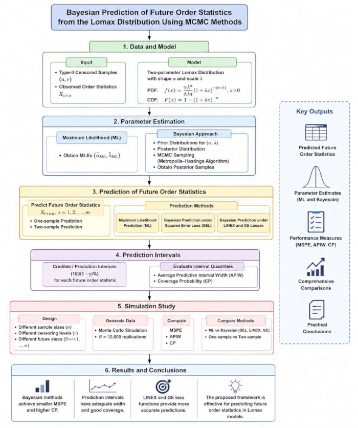
Figure 1: Analytical workflow for Bayesian prediction of future order statistics under Type-II censoring. Flowchart illustrating the analytical procedure used in this study. The workflow includes the generation of Type-II censored samples from the two-parameter Lomax distribution, construction of the predictive likelihood, parameter estimation using predictive maximum likelihood and Bayesian approaches, posterior sampling with the Metropolis–Hastings algorithm, the computation of Bayesian point predictors and predictive intervals under different loss functions, and the evaluation of predictive performance using Monte Carlo simulation. Please click here to view a larger version of this figure.

2. Lomax distribution

The two-parameter Lomax (Pareto Type II) distribution was used to model lifetime data because of its flexibility in representing heavy-tailed behavior. A random variable X was assumed to follow a Lomax distribution with a shape parameter ν > 0 and scale parameter β > 0, denoted by X ~ Lomax(ν, β), if its cumulative distribution function (CDF) is given^1,7 :

. (1)

The corresponding probability density function (PDF) was given by⁴˒⁶

. (2)

Here, ν represented the shape parameter controlling the tail behavior of the distribution, whereas β represented the scale parameter.

3. Order statistics and censoring scheme

A random sample of size n was assumed to be drawn from the two-parameter Lomax distribution. The corresponding order statistics were denoted by¹⁹˒²⁰:

. (3)

Under the Type-II censoring scheme, only the first r ordered observations were assumed to be observed, where r < n. The observed sample was therefore expressed as²⁶˒²⁷

. (4)

The remaining order statistics were treated as future observations to be predicted.¹⁹˒²⁰

4. Prediction framework

Two prediction scenarios were considered¹⁹˒²⁷.

5. One-sample prediction

The first r order statistics, x_(1:n) < x_(2:n) < ⋯ < x_(r:n), were assumed to be observed, and the remaining future order statistics, x_(r+1:n), x_(r+2:n), …, x_(n:n), were predicted from the same sample. This scenario is commonly encountered in Type-II censored life-testing experiments¹¹.

6. Two-sample prediction

The second prediction scenario considered future order statistics from an independent sample drawn from the same Lomax distribution. Specifically, the objective was to predict the first m order statistics of the future sample using information from the observed Type-II censored sample¹⁰˒¹¹˒¹⁹˒²⁷.

7. Prediction intervals

A 100(1 − α)% prediction interval for a future random variable Y was defined as²⁶˒³⁶

where L(X) and U(X) denote the lower and upper prediction limits, respectively.

8. Maximum likelihood prediction for future order statistics

Predictive maximum likelihood estimation was used as the classical prediction method. Let X_(1:n), X_(2:n), …, X_(r:n) denote the observed order statistics from a sample of size n, and let X_(s:n), where r < s ≤ n, denote the future order statistic to be predicted. The predictive likelihood function was defined as¹⁹˒²⁷

 (6)

where

.

and x₁ < x₂ < ⋯ < x_r < x_s.

Substituting the Lomax probability density and cumulative distribution functions into Equation (6) yielded the predictive likelihood function¹˒⁷

. (8)

The corresponding log-predictive likelihood was then obtained as⁹˒¹⁹

. (9)

The predictive maximum likelihood estimates of β, ν, and the future order statistic x_s were obtained by solving

. (10)

The expanded estimating equations are given in Equation (11).

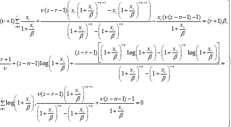   (11)

Because this system has no closed-form solution, the predictive maximum likelihood estimates  were obtained numerically.

9. Numerical implementation and algorithm

Because the nonlinear system in Equation (10) has no closed-form solution, the predictive maximum likelihood estimates (PMLEs) were obtained numerically¹²˒¹⁴. The system was solved using the FindRoot function with initial values β⁽⁰⁾, ν⁽⁰⁾, and x_s⁽⁰⁾. Iterations continued until the convergence criterion

was satisfied.

1. Asymptotic inference
   The asymptotic variance–covariance matrix of the PMLEs was obtained from the observed information matrix³²˒³⁸
   
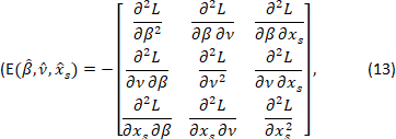
   evaluated at the PMLEs. The variance–covariance matrix was then computed as
   
2. Asymptotic predictive confidence intervals
   Under standard regularity conditions, the PMLEs were assumed to follow an asymptotic multivariate normal distribution.³⁶˒³⁸ Approximate predictive confidence intervals were therefore computed as
   
   where z_α/2 denotes the upper α/2 quantile of the standard normal distribution.

10. Bayesian prediction for future order statistics

A Bayesian framework was developed to predict the future order statistic X_(s:n) based on the observed sample x = (x_(1:n), …, x_(r:n)). Independent Gamma prior distributions were assigned to the positive parameters β and ν.¹⁰˒²⁷

. (16)

. (17)

Weakly informative hyperparameters were specified as ζ₁ = ω₁ = 0.35 and ζ₂ = ω₂ = 0.45, allowing the observed data to dominate the posterior inference while preserving parameter positivity. The resulting joint prior distribution was

. (18)

The future order statistic x_s was treated as a future random variable rather than an unknown model parameter; therefore, no prior distribution was assigned to x_s. Combining the joint prior with the predictive likelihood yielded the posterior distribution¹⁵˒¹⁸.

. (19)

Substituting the explicit forms, the normalized posterior density becomes

. (20)

Where

. (21)

The Bayesian predictive density of the future order statistic was then obtained by integrating over the posterior distribution²⁶˒¹⁶

. (22)

11. Bayesian point prediction

The Bayesian point predictor of X_(s:n) was obtained by minimizing the posterior expected loss under the posterior predictive distribution. Because the predictive density involved intractable integrals, posterior expectations were approximated using Markov Chain Monte Carlo (MCMC) samples generated after discarding the burn-in period¹⁴˒²⁸.

Let X_s^(j), j = 1, …, M, denote the retained MCMC samples.

12. Squared error loss (SEL)

Under the squared error loss (SEL) function, the Bayesian point predictor was given by the posterior mean¹⁰˒³⁶.

. (23)

13. LINEX Loss

Under the LINEX loss function, the Bayesian point predictor was computed as¹⁰

. (24)

14. General entropy loss

Under the general entropy (GE) loss function, the Bayesian point predictor was computed as¹¹˒²⁷

. (25)

15. Bayesian predictive intervals

A 100(1 − γ)% Bayesian predictive interval was obtained from the posterior predictive distribution.²⁶˒¹⁶ The interval limits satisfied

. (26)

The lower and upper prediction limits were estimated from the corresponding posterior predictive quantiles of the retained MCMC samples.

16. Comparison criteria

Predictive performance was evaluated using three criteria: mean squared prediction error (MSPE), average predictive interval width (APIW), and coverage probability (CP)³²˒³³˒³⁸.

1. Mean Squared Prediction Error (MSPE)
   The MSPE was calculated as
   . (27)
2. Average Predictive Interval Width (APIW)
   The APIW was calculated as³²˒³⁸
   .(28)

17. Coverage probability (CP)

Coverage probability was calculated as³³˒³⁸

. (29)

where I(·) denotes the indicator function.

18. Simulation algorithm and numerical procedures

A Monte Carlo simulation study was conducted to compare the Bayesian and predictive maximum likelihood methods under different sample sizes and Type-II censoring schemes. Random samples were generated from the two-parameter Lomax distribution using the inverse transformation method, and Type-II censoring was applied to obtain the observed order statistics. Future order statistics were then predicted using the predictive maximum likelihood method and the Bayesian approaches under the squared error (SEL), LINEX, and general entropy (GE) loss functions¹⁴˒²⁴.

Predictive maximum likelihood estimates were obtained by numerically solving the nonlinear equations described in Section 6. Bayesian inference was performed using the Metropolis–Hastings MCMC algorithm¹⁴˒²⁸. The Markov chain was initialized with β⁽⁰⁾ = 1.0 and ν⁽⁰⁾ = 1.5, using independent normal random-walk proposal distributions, β^* ~ N(β^(k), σ_β²), ν^* ~ N(ν^(k), σ_ν²),

with proposal standard deviations σ_β = 0.25 and σ_ν = 0.30.²⁹

For each simulation scenario, M = 11,000 MCMC iterations were generated, with the first M₀ = 1,000 discarded as burn-in. Convergence was assessed using a tolerance of 10⁻⁶ together with visual inspection of trace plots. Acceptance rates ranged from 27% to 34%, indicating satisfactory mixing of the Markov chains. Posterior samples obtained after burn-in were used to compute Bayesian point predictors and predictive intervals.

Each simulation scenario was replicated 10,000 times. Predictive performance was evaluated using the MSPE, APIW, and CP criteria³³˒³⁸. The numerical results are presented in Tables 1–4.

Method	Eβ	Eν	Predicted Future Values (xs)						MSPE	APIW	CP
			S=15	S=16	S=17	S=18	S=19	S=20
ML	2.1245	1.621	2.4102	2.5321	2.6841	2.851	3.0542	3.312	0.1542	2.4512	0.938
Bay-SEL	2.0582	1.5642	2.3851	2.5184	2.6512	2.8105	2.9981	3.2541	0.1251	2.2154	0.951
Bay-LINEX	2.0315	1.5381	2.371	2.5052	2.6391	2.7984	2.9812	3.2215	0.1182	2.1985	0.952
Bay-GE	2.0422	1.5495	2.3792	2.511	2.645	2.8012	2.9895	3.2381	0.1204	2.201	0.953

Table 1: Predictive performance of maximum likelihood and Bayesian methods for future order statistics under the Type-II censoring scheme (n = 20, r = 14). Parameter estimates, predicted future order statistics, mean squared prediction error (MSPE), average predictive interval width (APIW), and coverage probability (CP) obtained using predictive maximum likelihood (ML) and Bayesian methods under squared error loss (SEL), LINEX loss, and general entropy (GE) loss.Abbreviations: ML, predictive maximum likelihood; SEL, squared error loss; LINEX, linear exponential loss; GE, general entropy loss; MSPE, mean squared prediction error; APIW, average predictive interval width; CP, coverage probability.

Method	Eβ	Eν	Predicted Future Values (xs)					MSPE	APIW	CP
			S=46	S=47	S=48	S=49	S=50
ML	2.0412	1.5482	3.4215	3.551	3.7124	3.9215	4.215	0.0498	1.8214	0.949
Bay-SEL	2.0185	1.5212	3.4152	3.5381	3.6952	3.8991	4.1952	0.0382	1.7102	0.958
Bay-LINEX	2.0092	1.5085	3.4091	3.5302	3.6881	3.8812	4.1881	0.0351	1.6952	0.959
Bay-GE	2.0134	1.5142	3.4123	3.5345	3.691	3.8904	4.191	0.0368	1.7015	0.96

Table 2: Predictive performance of maximum likelihood and Bayesian methods for future order statistics under the Type-II censoring scheme (n = 50,r = 45). Comparison of parameter estimates, predicted future order statistics, MSPE, APIW, and CP for predictive maximum likelihood and Bayesian prediction methods under the moderate-sample simulation scenario.

Method	Eβ	Eν	Predicted Future Values (xs)					MSPE	APIW	CP
			S=96	S=97	S=98	S=99	S=100
ML	2.0214	1.5225	4.2581	4.3812	4.5912	4.881	5.4215	0.0285	1.5214	0.952
Bay-SEL	2.0091	1.5112	4.2514	4.3705	4.5801	4.8652	5.4012	0.0215	1.4521	0.96
Bay-LINEX	2.0042	1.5052	4.2482	4.3651	4.5752	4.8581	5.3952	0.0198	1.4402	0.962
Bay-GE	2.0061	1.5085	4.2505	4.3682	4.5781	4.861	5.3985	0.0205	1.4485	0.961

Table 3: Predictive performance of maximum likelihood and Bayesian methods for future order statistics under the Type-II censoring scheme (n = 100, r = 95). Comparison of parameter estimates, predicted future order statistics, MSPE, APIW, and CP for predictive maximum likelihood and Bayesian prediction methods under the large-sample simulation scenario.

Estimation Method	Estimates		Order (s)	Actual (xs)	Pred. xs	95% Pred. Interval		Width (W)	Error (ER)	CP (%)
	β	ν				Lower	Upper
ML Estimation	1.245	0.8921	s = 16	4.5	4.5125	3.211	5.814	2.603	0.0125	0.941
			s = 17	4.7	4.7215	3.421	6.022	2.601	0.0215	0.942
			s = 18	5	5.0488	3.5852	6.3172	2.732	0.0488	0.944
			s = 19	5.2	5.2159	3.7501	6.6181	2.868	0.0159	0.941
			s = 20	5.5	5.6712	4.1205	7.2219	3.1014	0.1712	0.935
Bayesian (SEL)	1.3102	0.9155	s = 16	4.5	4.5824	3.3215	5.8433	2.5218	0.0824	0.951
			s = 17	4.7	4.8104	3.5512	6.0696	2.5184	0.1104	0.952
			s = 18	5	5.0612	3.7251	6.3973	2.6722	0.0612	0.954
			s = 19	5.2	5.3125	3.911	6.714	2.803	0.1125	0.955
			s = 20	5.5	5.8124	4.3501	7.4105	3.0604	0.3124	0.948
Bayesian (LINEX)	1.308	0.9132	s = 16	4.5	4.571	3.3104	5.8318	2.5214	0.071	0.954
			s = 17	4.7	4.7952	3.541	6.0494	2.5084	0.0952	0.955
			s = 18	5	5.041	3.7142	6.3678	2.6536	0.041	0.958
			s = 19	5.2	5.2912	3.9002	6.6822	2.782	0.0912	0.959
			s = 20	5.5	5.7412	4.3412	7.3982	3.057	0.2412	0.952
Bayesian (GE)	1.3115	0.9168	s = 16	4.5	4.5912	3.3284	5.854	2.5256	0.0912	0.952
			s = 17	4.7	4.8051	3.5482	6.062	2.5138	0.1051	0.953
			s = 18	5	5.0552	3.7201	6.3903	2.6702	0.0552	0.956
			s = 19	5.2	5.3051	3.9054	6.7048	2.7994	0.1051	0.957
			s = 20	5.5	5.7985	4.345	7.401	3.056	0.2985	0.951

Table 4: Comparison of predictive estimates and 95% prediction intervals for future order statistics under the Type-II censoring scheme (n = 20,r = 15). Comparison of predictive maximum likelihood and Bayesian methods based on parameter estimates, predicted future order statistics, 95% prediction intervals, interval widths, prediction errors, and coverage probabilities for an additional Type-II censoring scenario.

19. Data generation

Random samples were generated from the two-parameter Lomax distribution using the inverse transformation method.¹˒⁷˒³⁸˒³⁹ Uniform random variables U₁, U₂, …, U_n ~ U(0,1) were transformed according to X_i = β[(1 − U_i)^−1/ν − 1], i = 1, 2, …, n,

where ν and β denote the shape and scale parameters, respectively. The generated observations were sorted to obtain the order statistics X_(1:n) < X_(2:n) < ⋯ < X_(n:n).

The first r order statistics were retained as the observed Type-II censored sample, and the s-the order statistic (r < s ≤ n) was treated as the future observation to be predicted.

20. Evaluation metrics

For each simulation replication, Bayesian and predictive maximum likelihood predictors, together with their prediction intervals, were computed. Predictive performance was evaluated using the mean squared prediction error (MSPE), average predictive interval width (APIW), and coverage probability (CP), as defined in Equations (27)–(29).

21. Computational implementation

All numerical computations and simulation procedures were performed using Wolfram Mathematica.

결과

A Monte Carlo simulation study was conducted to compare the predictive performance of the Bayesian and predictive maximum likelihood (PML) methods for future order statistics from the two-parameter Lomax distribution under different sample sizes and Type-II censoring schemes. Predictive performance was evaluated using the mean squared prediction error (MSPE), average predictive interval width (APIW), and coverage probability (CP). Tables 1–4 summarize the parameter estimates, predicted future order statistics, and corresponding predictive performance measures.

Figure 2 presents representative trace plots of the Metropolis–Hastings Markov chains for the shape parameter α (panel A) and the scale parameter β (panel B), respectively. In both panels, the vertical dashed line indicates the burn-in period, and the horizontal dashed line denotes the true parameter value. After burn-in, the chains fluctuated around the true parameter values without apparent trends, indicating stable mixing and satisfactory convergence. Acceptance rates ranging from 27% to 34% further supported the efficiency of the sampling algorithm.

For the small-sample scenario (n = 20, r = 14), Table 1 shows that the Bayesian-LINEX predictor achieved the lowest MSPE (0.1182), representing an improvement of approximately 23.3% over the PML method (0.1542). The Bayesian methods also produced narrower predictive intervals and slightly higher coverage probabilities than the PML approach.

For the moderate sample size (n = 50, r = 45), Table 2 showed a similar pattern. The Bayesian-LINEX predictor yielded the lowest MSPE (0.0351), corresponding to an improvement of approximately 29.5% over the PML method, while maintaining narrower predictive intervals and higher coverage probabilities. The Bayesian-GE method also demonstrated competitive predictive performance.

For the large-sample scenario (n = 100, r = 95), Table 3 demonstrated improved predictive accuracy for all methods. The Bayesian-LINEX predictor again achieved the lowest MSPE (0.0198), representing an improvement of approximately 30.5% over the PML method. Bayesian predictors also produced narrower predictive intervals with slightly higher coverage probabilities.

Table 4 presents an additional simulation scenario (n = 20, r = 15). The Bayesian prediction methods consistently produced lower prediction errors, narrower predictive intervals, and higher coverage probabilities than the predictive maximum likelihood approach under this censoring configuration.

Overall, the simulation results demonstrated that the Bayesian prediction methods consistently outperformed the predictive maximum likelihood approach across all investigated scenarios. Among the Bayesian methods, the LINEX loss function generally achieved the lowest MSPE, whereas the Bayesian predictors as a whole provided narrower predictive intervals while maintaining satisfactory coverage probabilities.

Data availability:

The raw Monte Carlo simulation data underlying the results reported in Tables 1–4 are provided as Supplementary File 1 (ZIP archive), which contains the Microsoft Excel (.xlsx) source data files for each simulation scenario.

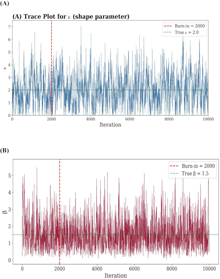
Figure 2: Representative Metropolis–Hastings trace plots for Bayesian estimation of the Lomax distribution parameters. (A) Trace plot for the shape parameter α. (B) Trace plot for the scale parameter β. The vertical dashed line indicates the burn-in period, and the horizontal dashed line denotes the true parameter value used in the simulation. The post-burn-in samples fluctuate around the true parameter values without noticeable trends, indicating satisfactory mixing and convergence of the Markov chains. Please click here to view a larger version of this figure.

Supplementary File 1: Raw Monte Carlo simulation data supporting Tables 1–4.Please click here to download this file.

토론

In conclusion, this study developed a Bayesian predictive framework for future order statistics from the two-parameter Lomax distribution under Type-II censoring by integrating Bayesian predictive inference with the Metropolis–Hastings Markov Chain Monte Carlo (MCMC) algorithm. The proposed methodology was investigated under the squared error (SEL), LINEX, and general entropy (GE) loss functions and compared with the predictive maximum likelihood approach. The simulation study demonstrated that the Bayesian predictive procedures provided competitive predictive performance across different sample sizes and censoring configurations, while the LINEX and general entropy loss functions frequently yielded lower prediction errors together with satisfactory predictive interval characteristics. The findings highlight the practical importance of incorporating parameter uncertainty into predictive inference for censored lifetime data. Unlike classical predictive maximum likelihood methods, the Bayesian framework provides complete posterior predictive distributions, allowing both point prediction and uncertainty quantification within a unified probabilistic framework. The observed improvements in prediction accuracy, interval width, and coverage probability across all investigated scenarios indicate that the proposed approach offers a reliable alternative for predicting future order statistics, particularly in situations where censored observations and relatively small sample sizes are encountered. From an application perspective, the proposed methodology has potential relevance in reliability engineering, life-testing experiments, maintenance planning, survival analysis, actuarial science, and risk assessment, where accurate prediction of future failure times is essential for decision-making. The flexibility of the Bayesian framework also allows prior information to be incorporated whenever such information is available, making the approach suitable for practical reliability studies in which historical knowledge or expert opinion may complement observed data. By explicitly accounting for parameter uncertainty, the proposed framework provides a unified approach for Bayesian prediction of future order statistics and extends the existing literature on predictive inference for censored lifetime data. The proposed methodology may serve as a useful framework for reliability and lifetime data analysis in applications where uncertainty quantification is of practical importance. Although the Metropolis–Hastings algorithm provided satisfactory convergence and stable predictive performance, alternative Bayesian computational strategies, including Gibbs sampling, Hamiltonian Monte Carlo, Sequential Monte Carlo methods, or variational Bayesian approaches, may provide computational advantages for more complex predictive models or higher-dimensional parameter spaces. Comparative investigations of these approaches would further clarify their relative efficiency and predictive performance. Although the present study is limited to the two-parameter Lomax distribution under Type-II censoring and simulation-based evaluation, it provides a solid foundation for further methodological developments. Future research will focus on extending the proposed framework to more general lifetime distributions, alternative censoring schemes, real-world datasets, different prior specifications, and more advanced Bayesian computational techniques, as well as conducting broader comparative studies with alternative Bayesian computational approaches.

재료

이 논문에 사용된 재료 목록

이름	회사	카탈로그 번호	댓글
Computational software (Bayesian estimation and MCMC simulations)	Wolfram Research, Inc.	Mathematica Version 12.0	Used for parameter estimation, MCMC implementation, posterior sampling, and numerical computations.
Computational software (symbolic derivations)	Wolfram Research, Inc.	Mathematica Version 12.0	Used for symbolic manipulations and derivation of predictive formulas.
Equation editor	Microsoft Corporation	Microsoft Word Equation Editor	Used for preparation and formatting of mathematical expressions and equations.
Personal computer/workstation	HP Inc.	N/A	Used to perform numerical calculations and Monte Carlo simulation experiments.
Simulated Type-II censored datasets	Generated in this study	N/A	Artificial datasets generated according to the two-parameter Lomax distribution for simulation experiments.