Quantifying the Functional Effect of Transmural Interpolation Strategies on Atrial Wave Propagation Using a Custom Open-Source Pipeline

Samenvatting

This protocol describes a comprehensive, open-source pipeline for reconstructing patient-specific 3D transmural fiber orientation in the human left atrium from clinical computed tomography data.

Samenvatting

Atrial fibrillation (AF) management increasingly relies on patient-specific computational modeling to simulate arrhythmia mechanisms and optimize ablation strategies. However, predictive reliability is strongly influenced by accurate reconstruction of myocardial fiber architecture, which governs electrical anisotropy. Because patient-specific atrial fiber orientations cannot currently be acquired reliably in vivo using diffusion tensor magnetic resonance imaging (DT-MRI), alternative computational mapping strategies are required. This protocol presents a comprehensive, open-source pipeline for constructing patient-specific 3D models of the human left atrium with explicit transmural fiber reconstruction from high-resolution clinical computed tomography (CT) data. The methodology extends the Universal Atrial Coordinate (UAC) framework into the volumetric domain by solving the Laplace–Dirichlet problem to derive a continuous transmural coordinate. This enables transfer of atlas-based fiber orientations and subsequent interpolation across the atrial wall. Linear and threshold-based transmural interpolation strategies are quantitatively compared, and their effects on fiber orientation and macroscopic wavefront propagation are evaluated. Across all six models, the mean angular deviation between interpolation methods was 8.06 ± 1.13°. Electrophysiological simulations demonstrate that the choice of interpolation delayed activation in Region 1 by 2.0 ± 0.6 ms, corresponding to 6.1 ± 1.5 ms (p = 0.031 for both comparisons). The open-source pipeline and patient-specific CT-based atrial models provide a reproducible framework for evaluating the functional effects of transmural fiber reconstruction strategies.

Inleiding

Atrial fibrillation (AF) remains the most prevalent sustained cardiac arrhythmia, imposing a substantial burden on global health through increased risks of stroke, heart failure, and mortality^1,2. Catheter ablation, which aims to electrically isolate arrhythmogenic triggers, is currently the cornerstone of interventional AF management. Despite its widespread adoption, long-term procedural success rates remain modest, largely driven by considerable inter-patient variability in atrial anatomy and the underlying electrophysiological substrate^2,3. Recent computational studies have further emphasized how sex- and disease-specific anatomical differences significantly influence cardiac electrophysiology, underscoring the critical need for highly adaptable and anatomically precise modeling frameworks⁴. Computational modeling has emerged as an innovative paradigm to address this complexity, enabling the development of patient-specific models capable of simulating arrhythmia mechanisms and refining therapeutic strategies^5,6,7. However, the clinical utility and predictive reliability of these frameworks can be significantly influenced by the anatomical and microstructural fidelity of the underlying computational meshes, as inaccuracies in geometric representation or fiber orientation can introduce uncertainties in simulation outcomes^8,9.

Myocardial fiber architecture is a primary determinant of atrial electrophysiology^10,11. Cardiac tissue exhibits strong electrical anisotropy, with conduction velocities significantly faster along the fiber axis than across it. This directional dependence controls wavefront curvature, dictates the spatial distribution of conduction block, and critically influences the initiation and stability of re-entrant circuits during AF. Ignoring or oversimplifying fiber orientation in computational models leads to substantial deviations in simulated activation sequences and virtual ablation outcomes^6,12. Therefore, accurate reconstruction of the three-dimensional (3D) fiber field is a fundamental requirement for physiologically realistic propagation modeling.

Despite its importance, acquiring patient-specific atrial fiber orientations in vivo remains technically unfeasible. Diffusion tensor magnetic resonance imaging (DT-MRI), the gold standard for mapping myocardial microstructure, cannot reliably resolve the thin, rapidly contracting atrial walls in routine clinical practice^13,14. To overcome this limitation, contemporary modeling pipelines rely on alternative strategies. Rule-based algorithms generate synthetic fiber fields but often produce overly smooth distributions that suppress inter-individual microstructural variability¹⁵. Image-based registration techniques deform high-resolution ex vivo fiber atlases to match patient geometries, but these are highly sensitive to landmark placement and prone to angular mismatches at complex topological junctions^16,17. Recent innovations have introduced Universal Atrial Coordinate (UAC) systems to standardize surface fiber mapping across diverse anatomies¹⁸.

However, a major bottleneck remains in resolving transmural fiber variation. The left atrial wall is exceptionally thin, typically 1 – 4 mm, and exhibits complex, regionally heterogeneous transmural rotation, including abrupt, near-orthogonal transitions between layers^13,19,20. Existing volumetric models frequently assume uniform fiber orientation across the wall thickness or rely on simplistic interpolation methods. These limitations compromise the accuracy of modeling transmural conduction and re-entry dynamics, which are key factors in arrhythmia maintenance^20,21.

To bridge this gap, this study presents and rigorously evaluates a computational pipeline for constructing personalized 3D models of the left atrium with explicit transmural fiber reconstruction. The foundational fiber orientations are derived from the Human Atrial Fibre Atlas, which was originally constructed from high-resolution ex vivo DT-MRI data of human atria^13,22. By integrating patient-specific anatomical data derived from clinical computed tomography (CT) with a geometry-constrained interpolation framework, this approach generates a continuous, depth-resolved fiber orientation field.

The primary methodological contribution of this work is the quantitative comparison of distinct transmural interpolation strategies, linear versus threshold-based, and the evaluation of their direct, measurable impact on macroscopic wavefront propagation. In this study, the reconstruction framework is described, the interpolated anisotropy is validated against established electrophysiological principles, and its utility is demonstrated by quantifying Local Activation Time (LAT) differences induced by varying interpolation methods. Furthermore, by releasing the fully open-source processing pipeline alongside high-resolution, patient-specific CT-based atrial models, this work contributes to the growing ecosystem of public virtual cohorts and open computational resources⁴. This provides the research community with a mathematically rigorous, reproducible alternative to simplistic fiber assumptions, supporting the transition toward truly personalized patient-specific models for precision-guided therapeutic planning^23,24.

Protocol

The study was conducted in accordance with the Declaration of Helsinki and approved by the Ethics Committee of the M.F. Vladimirsky Moscow Regional Clinical Research Institute (official approval reference: Protocol No. 7, dated 18 April 2024). Voluntary written informed consent was obtained from all participants prior to enrollment. The research tools used in this protocol are listed in the Table of Materials.

1. Construction of a patient-specific 3D atrial geometry from tomographic imaging data

1. Acquire patient-specific atrial images using high-resolution cardiac computed tomography (CT).
   NOTE: The study cohort comprised 6 patients, including 5 males and 1 female, aged 57–66 years. All patients had a documented clinical history of atrial fibrillation that had progressed to a persistent form lasting ≥3 years. Volumetric datasets were reconstructed using a high-spatial-frequency cardiac kernel, yielding a spatial resolution of 0.4 × 0.4 × 0.625 mm³.
2. Process cardiac CT volumes in Nearly Raw Raster Data (.nrrd) format using 3D Slicer (v5.8.1)²⁵. Correct voxel anisotropy via interpolated cropping to achieve isotropic resolution. Perform semi-automated segmentation of the cardiac chambers using the “Grow from Seeds” algorithm. Refine the left atrial segmentation by manual editing and perform threshold-based endocardial surface extraction to separate the endocardial, epicardial, and myocardial wall surfaces. Export the final geometric models of the epicardial and endocardial layers and the atrial wall in .vtk format for downstream computational modeling.
   NOTE: The complete step-by-step segmentation pipeline with illustrative figures is provided in Supplementary File 1 Section 1.
3. Convert the resulting model to openCARP format using the Meshtool utility, then generate a volumetric finite-element mesh using the Constrained Delaunay Tetrahedralisation method²⁶. Ensure that the initial surface shell mesh is watertight, closed, free of holes, non-self-intersecting, and has consistent normals. Obtain the final 3D atrial mesh upon completion of the full segmentation and reconstruction pipeline (Figure 1).
   NOTE: The following steps in the protocol are general and apply to both CT and magnetic resonance imaging (MRI) data. Additional information and visual results of the MRI application are provided in Supplementary File 1 Section 1.

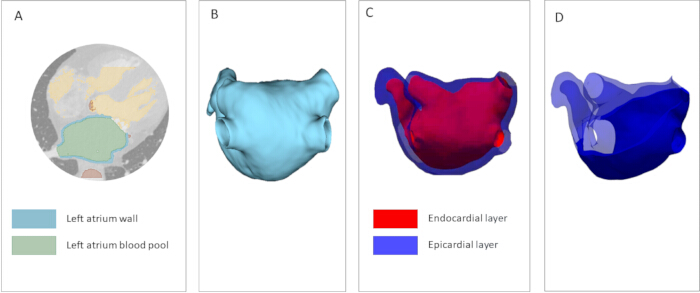
Figure 1: Construction of a patient-specific 3D atrial geometry mesh from computed tomography (CT) data. (A) Segmentation of patient-specific cardiac structures from high-resolution CT imaging. Green denotes the blood pool; blue indicates the left atrial wall. (B) Atrial segmentation serves as the foundation for the computational model. (C) Epicardial and endocardial layers of the model atrium are represented as shell surfaces. (D) Volumetric atrial model. A mesh cross-section displays the solid tetrahedralized atrial wall. Please click here to view a larger version of this figure.

2. Construction of the universal atrial coordinate (UAC) system for surface parametrization

NOTE: All steps in this section must be performed separately for the epicardial and endocardial layers.

1. Annotate atrial landmarks. Select coordinates for the following anatomical landmarks: the ostia of the four pulmonary veins (right superior, right inferior, left superior, and left inferior), and the apex and base of the left atrial appendage (Figure 2A). Consider variation in the precise placement of these points to have negligible impact on the final segmentation. 
2. Additionally, select three auxiliary points: at the junction of the right superior pulmonary vein with the LA body (RSPV-LA), at the junction of the left superior pulmonary vein with the LA body (LSPV-LA), on the interatrial septum (Figure 2B). Choose landmarks in the vicinity of their anatomically optimal position: the anterior wall point near the appendage base, and the pulmonary vein points near the atrial roof (where anterior/posterior wall separation is most clearly defined).
3. Select a threshold value φ _threshold to define the anatomical boundary. Areas with φ > φ _threshold are considered to belong to the target structure. For pulmonary veins, φ _threshold = 0.75, and for atrial appendage: φ _threshold = 0.35 (Figure 2C). Extract the surface elements and vertices corresponding to these structures, annotate them with appropriate tags, and reintegrate them into the mesh (Figure 2D).
4. Solve Laplace's equation on the mesh surface:
   
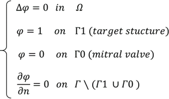
5. where φ ∈ [0,1] is the scalar coordinate field, Ω is the volumetric mesh domain, Г1 is the boundary of the target structure (pulmonary vein ostia or appendage base, Г0 is the mitral valve annulus boundary, and, ∂φ /∂n = 0 denotes the no-flux Neumann condition.
6. Conduct a comprehensive sensitivity analysis to quantitatively assess the impact of landmark variation on the fiber field (Figure 3). For more detailed instructions on how to place points and evaluate sensitivity to their position, see Supplementary File 1 Section 2.
7. Perform a cut of the atrial surface along the shortest geodesic paths from the selected reference points (RSPV-LA and LSPV-LA) to the mitral valve annulus, passing through the user-defined septal landmark, to define the α coordinate (Figure 4).
8. Subsequently solve Laplace's equation to define the posterior-anterior coordinate β. Assign Dirichlet boundary conditions β = 0 on one cut edge and β = 1 on the opposite edge.
9. For both coordinates, solve Laplace's equation Δψ = 0 with boundary conditions ψ = 0 on one boundary and ψ = 1 on the other. Rescale the β coordinate as β = 0.5 ⋅ ψ on the posterior wall and β = 1 - 0.5⋅ψ on the anterior wall. The final output is a 2D representation of the epicardial and endocardial atrial surfaces (Figure 5).
10. Repeat the aforementioned steps for the reference anisotropic models of the epicardial and endocardial layers derived from the Human Atrial Fibre Atlas^13,22. Average the resulting fields to ensure standardization.

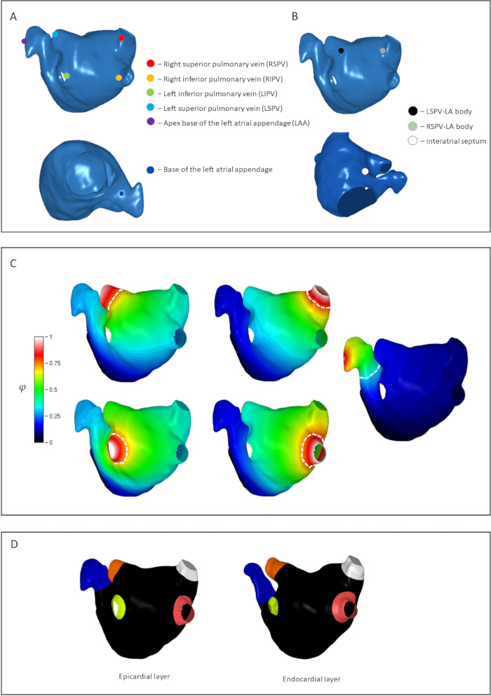
Figure 2: Mapping of key anatomical structures of the left atrium, illustrated for the epicardial surface. (A) Selection of six coordinates for tagging pulmonary vein and atrial appendage regions. The anatomical landmarks shown are the ostia of the pulmonary veins (right superior, right inferior, left superior, and left inferior) and the apex and base of the left atrial appendage. (B) Selection of three reference points for surface parametrization. Points are indicated at the junction of the right superior pulmonary vein with the atrial body, at the junction of the left superior pulmonary vein with the atrial body, and on the interatrial septum. (C) Results of Laplace equation solutions on the mesh surface for all target structures. White dashed lines indicate threshold values for the veins and appendage; regions exceeding these thresholds are classified as belonging to the corresponding anatomical structure. (D) Labeled epicardial and endocardial surfaces of the patient-specific atrium. Please click here to view a larger version of this figure.

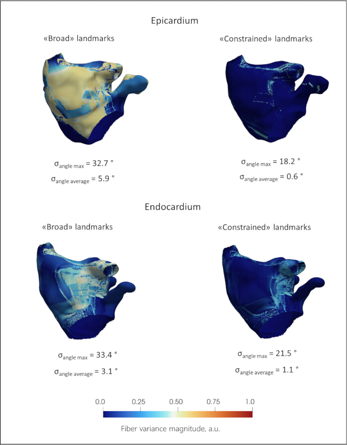
Figure 3: Sensitivity analysis of fiber orientation transfer to auxiliary landmark placement variability. The color maps represent fiber variance magnitude in arbitrary units. σ_angle max denotes the maximum standard deviation of the angle for a given atrial model, and σ_angle average denotes the average value of the deviation angles for a given model. Upper row: Epicardial surface. Under broad landmark placement, σ_angle max reaches 32.7°, with a mean deviation, σ_angle average, of 5.9°. When landmarks are constrained to their optimal anatomical neighborhood, σ_angle max decreases to 18.2° and σ_angle average decreases to 0.6°. Lower row: Endocardial surface. Under broad landmark placement, σ_angle max is 33.4°, with σ_angle average of 3.1°. With constrained landmark placement, σ_angle max decreases to 21.5° and σ_angle average decreases to 1.1°. Please click here to view a larger version of this figure.

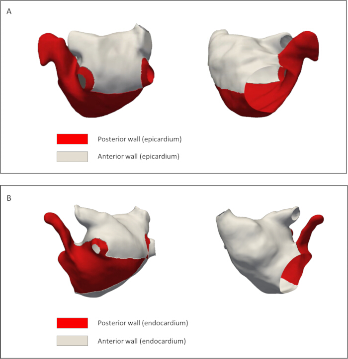
Figure 4: Geodesic cutting paths for Universal Atrial Coordinate (UAC) parametrization of the left atrium. (A) Epicardial surface and (B) endocardial surface, both shown in posteroanterior view with anterior and posterior walls labeled. Edges indicate the shortest geodesic paths used to define the septal-lateral coordinate boundary. The anterior wall of the atrium is denoted in white, and the posterior wall is denoted in red. Please click here to view a larger version of this figure.

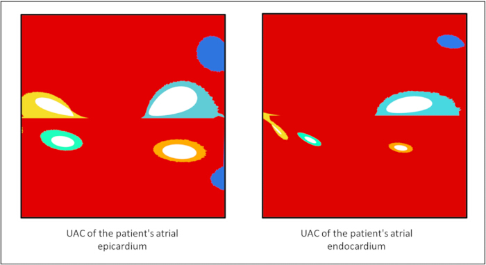
Figure 5: Two-dimensional representation of the patient-specific Universal Atrial Coordinate (UAC) system for the epicardial and endocardial atrial surfaces. Anatomical structures, including the pulmonary vein ostia and atrial appendage, are color-coded to indicate correspondence across surfaces. Please click here to view a larger version of this figure.

3. Transfer of fibers from the atlas to the model atrium.

1. To transfer the fiber architecture from the atlas to the patient-specific geometry, utilize the Universal Atrial Coordinates (UAC) system.
   NOTE: Spatial transformations are based on the methodology¹⁸. Fiber orientation data for this atlas was constructed from high-resolution ex vivo diffusion tensor magnetic resonance imaging (DT-MRI) of human atria¹³. All the steps in this section must be performed for the epicardial and endocardial layers separately
2. Map fiber vectors based on their functional anatomical correspondence within the 2D parametric (α, β) space. Project fiber directions from the atlas into the UAC basis and assign to the target mesh elements via a nearest-neighbor search. Then map these vectors back to the patient's physical 3D space and normalize, ensuring a smooth, anatomically consistent anisotropy field that respects the local geometry.
3. For the detailed mathematical formulations of the barycentric interpolation, coordinate transformations, and finite element basis functions, refer to Supplementary File 1 Section 3. The resulting vector is normalized to unit length, yielding an anisotropy field that is consistent with the patient’s local geometry (Figure 6).

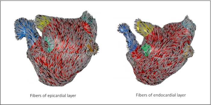
Figure 6: Anisotropic field of transferred fibers for the epicardial and endocardial surfaces. The vectors are color-coded to represent their local 3D orientation relative to a defined reference axis. Distinct anatomical structures, including the pulmonary vein ostia and the left atrial appendage, are highlighted in specific colors (blue, yellow, green, and orange) to indicate their anatomical correspondence across both layers. Please click here to view a larger version of this figure.

4. Restoration of transmural fiber orientation

NOTE: The next steps require 2D Unfolding of the endocardial and epicardial atrial surface in two orthogonal scalar fields α and β mapped with fiber fields from the Atlas, obtained after completing protocol Sections 2 and 3.

1. Introduce the continuous transmural coordinate γ field. Extract the 3D coordinates of the nodes forming the outer boundary of the volumetric mesh. Load the coordinates of the endocardial and epicardial surfaces of the reference atlas. Define a continuous normalized transmural coordinate, γ∈[0,1] by solving the Laplace equation ∇²γ=0 across the atrial wall thickness. Use the endocardial surface as the γ=0 boundary and the epicardial surface as the γ=1 boundary.
2. Map the surface (α,β) coordinates inward along the gradient of γ (Figure 7A). Extend the 2D surface parameterization into the 3D volumetric mesh to create a fully volumetric coordinate system and map the surface (α,β) coordinates inward along the gradient of γ. To do this, for each node on the volumetric surface, identify the nearest corresponding nodes on the endocardium and epicardium for each volumetric surface node in Cartesian space via a nearest-neighbor search (KD-tree, k=1), recording the Euclidean distances to both layers. 
3. Assign the (α,β) coordinates corresponding to the nearest endocardial node to each volumetric surface node. This ensures that every node or finite element within the myocardial wall possesses a unique, continuous scalar field (α,β,γ), called 3D UAC (Figure 7B).
4. Perform transmural fiber orientation mapping. Define the normalized transmural coordinate γ∈[0,1], where γ=0 corresponds to the endocardial surface and γ=1 corresponds to the epicardial surface.
5. Use traditional threshold interpolation methods, in which each point of the myocardium is assigned a direction depending on whether it is closer to the epicardium or endocardium.
6. Use the direct linear interpolation approach of three-dimensional Cartesian vectors. Choose the unit fiber direction vectors on the bounding surfaces: f^→_endo ∈ R³ - fiber orientation on endocardium, f^→_epi ∈ R³ - fiber orientation on epicardium. Prior to interpolation processe, evaluate the dot product of the endocardial and epicardial fiber vectors. If f^→_endo · f^→_epi < 0, the sign of the epicardial vector is flipped to ensure the shortest rotational path is taken, preventing artificial vector cancellation at the mid-wall. Obtain the fiber direction f (γ) at any point within the myocardial wall via linear interpolation in Cartesian space:
   
7. To preserve a unit direction vector, normalize the interpolated result:
   
   Yield a smooth, continuous, and topologically consistent scalar field(α,β,γ) throughout the entire atrial wall (Figure 7С). 

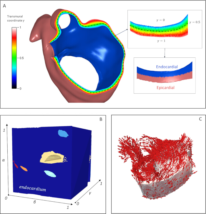
Figure 7: Construction of the 3D Universal Atrial Coordinate (UAC) system and transmural fiber orientation mapping. (A) Derivation of the continuous transmural coordinate γ via the Laplace–Dirichlet problem solution for each volumetric mesh element of the myocardial wall. The color map represents the normalized coordinate γ ∈ [0,1], where γ = 0 corresponds to the endocardial surface (blue), γ = 1 corresponds to the epicardial surface (red), and the mid-wall is indicated at γ = 0.5 by the dashed black line. (B) Constructed 3D UAC coordinate system (α, β, γ) visualized within the volumetric mesh domain. The axes represent normalized coordinates ranging from 0 – 1. The endocardial surface geometry is embedded within this 3D parametric space. (C) The resulting fiber orientation field is determined at any point within the myocardial wall and obtained by linear interpolation of atlas-derived fiber vectors along the γ coordinate. Red arrows represent the local 3D fiber-direction vectors mapped across the atrial geometry. Please click here to view a larger version of this figure.

5. Estimation of fiber orientation effects

1. Assess the fiber orientation alignment on patient-specific layers. Deform the epicardial and endocardial surfaces of the reference atrium from the atlas to match the geometry of the corresponding layers in the patient's atrium.
2. Apply affine transformations constrained by a set of anatomical landmarks, including the mitral valve annulus, pulmonary vein ostia, interatrial septum, and atrial appendage. Identify corresponding mesh vertices between the reference and patient-specific layers using a k-dimensional tree (KD-tree) algorithm with k = 1. 
3. Investigate spatial correspondence after fiber transfer from atlas to patient-specific geometry and quantify errors. Compute the orientation transfer error at each mesh vertex as the absolute angular difference as θ = min(|θ_t - θ_a|, π - |θ_t - θ_a|), restricting the range to [0, π/2], where θ_t and θ_a represent the inclination angles of the transferred and atlas-derived fiber orientations, respectively (Figure 8). Repeat this procedure independently for both the epicardial and endocardial surfaces.
   NOTE: As a quality-control metric, if the mean angular transfer error exceeds 30° or localized peaks exceed 45° in critical regions (e.g., pulmonary vein ostia, mitral valve annulus, left atrial appendage), manual refinement of the auxiliary landmark placement is recommended before proceeding to volumetric interpolation.
4. Evaluate the difference in the transmural directions of the fibers depending on the method of interpolation along the depth of the atrial wall (Figure 9). Assess the differences in fiber orientation between threshold-based and linear interpolation methods.
5. Calculate the angular deviation in fiber direction at each point within the atrial myocardium for a reconstructed model. Quantify the directional differences as angles of deviation ranging from 0 – 90 degrees (Figure 10A).
6. Investigate excitation wave propagation on the patient-specific atrial model. Using the openCARP v.12 software package²⁷, simulate the sinus rhythm in the atrium using both a reconstructed linearly interpolated fiber field and a control case with uniform fiber orientation to verify the presence of anisotropic effects (Figure 11).
7. Apply the pacing protocol consisting of 10 consecutive stimuli with the pacing cycle length 200 ms. Simulate the sinus rhythm in the atrium using both a reconstructed linearly interpolated fiber field and a reconstructed threshold fiber field to measure the difference in wavefront propagation (Figure 10B).
8. Perform electrophysiological simulations for both fiber architectures using the monodomain formulation with the Courtemanche-Ramirez-Nattel human atrial action potential model²⁸.
9. Apply the pacing protocol at the LA roof, proximal to the right pulmonary veins, consisting of 10 consecutive stimuli with the pacing cycle length progressively decreasing from 300 ms to 200 ms in 10 ms steps.
10. Following the 10th stimulus, compute local activation times (LATs) for each node across the atrial geometry. To quantify the regional conduction differences arising from the fiber transmural reconstruction methods, extract LATs from two regions exhibiting transmural fiber angular differences. Choose regions approximately equidistant from the pacing site that exhibit maximal transmural fiber divergence.
11. Model cardiac electrophysiological propagation at the tissue level using the monodomain equation, coupled with the Courtemanche human atrial cell model to describe the ionic currents:
    
    where Vm is the transmembrane potential, t is time, Cm​ is the specific membrane capacitance, Iion represents the total transmembrane ionic current density and Ist represents stimulation current, K1, IKur, Ito are the potassium currents, INa  is the fast sodium and ICaL is L-type calcium current.
12. Assign an effective conductivity tensor to the myocardial tissue with longitudinal conductivity σ_L = 0.4 S/m and transverse conductivity σ_T = 0.1 S/m. Solve the governing equations numerically with a time step of Δt = 20 µs. Execute the simulations under the specified hardware configuration, requiring approximately 1 h of computation time per 10 s of electrophysiological activity.
    NOTE: Additional patient-specific examples and supporting analyses for the segmentation, landmark sensitivity, fiber transfer, and electrophysiological comparisons are provided in Supplementary Figures 1–20.

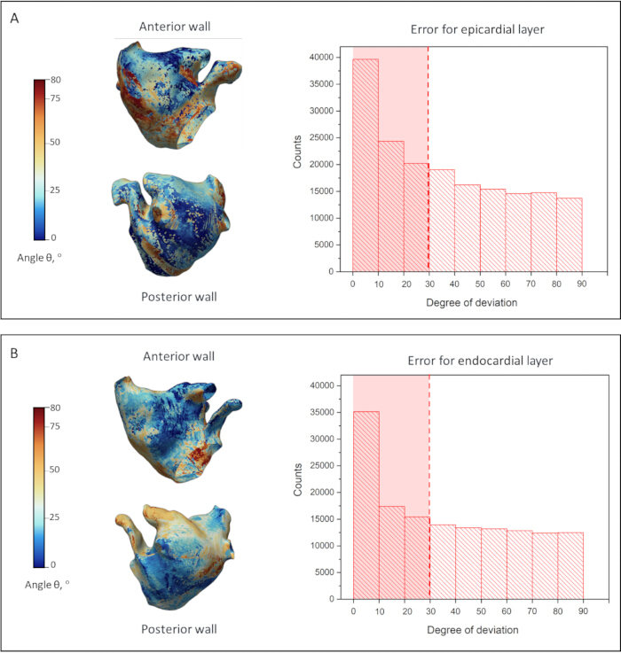
Figure 8: Validation of the fiber orientation transfer methodology. Comparison of reconstructed fiber orientations with atlas-derived orientations for the epicardium (A) and endocardium (B). The 3D surface maps, shown in anterior and posterior views, display the spatial distribution of the angular transfer error (θ), quantified as the angular difference between the original atlas-based and reconstructed fiber directions. The surface color scale ranges from 0° to 80°, while the accompanying histograms show the distribution of angular transfer errors across all mesh elements over the full 0°–90° range. The red dashed lines indicate the median error magnitude, 28.9° for the epicardial layer and 29.4° for the endocardial layer. Please click here to view a larger version of this figure.

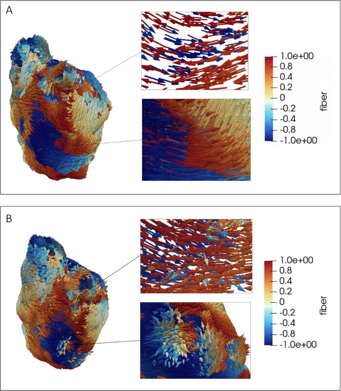
Figure 9: Evaluation of fiber orientation transfer from the surface into the myocardial wall depth. Two cases are presented: threshold-based (A) and linear (B) interpolation. The color map displays fiber directions relative to a defined reference axis, with the scalar component ranging from −1.0 to +1.0, where values near zero indicate fibers oriented perpendicular to the reference axis. The circled regions on the main 3D renderings indicate the anatomical locations from which the enlarged cross-sectional views are extracted, highlighting areas where epicardial and endocardial fibers are nearly orthogonal or oppositely directed. Particular attention is given to the transmural transition from the epicardium to the endocardium. Individual fiber orientations are explicitly rendered on the atrial surface geometry. Please click here to view a larger version of this figure.

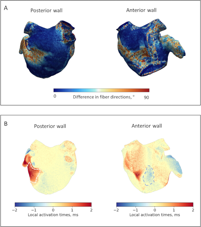
Figure 10. Quantitative comparison of transmural fiber interpolation methods and their functional impact on atrial electrophysiology for the representative model. (A) Spatial distribution of angular deviations in fiber orientation between threshold-based and linear interpolation methods. The color maps display the angular difference in fiber directions, ranging from 0° to 90°, calculated at each point within the atrial myocardium for posterior and anterior wall views. (B) Quantitative assessment of Local Activation Time (LAT) differences between threshold-based and linear interpolation methods across the posterior and anterior walls. The color maps represent the LAT difference in milliseconds, ranging from −2 to +2 ms, where positive values indicate regions where linear interpolation delays activation compared with threshold-based interpolation, and negative values indicate the opposite. White dashed lines outline Region 1, the lateral wall near the left pulmonary veins and left atrial appendage, and Region 2, the anterior wall adjacent to the mitral valve. These regions exhibit maximal transmural fiber divergence and statistically significant LAT differences across all models (p = 0.031). Please click here to view a larger version of this figure.

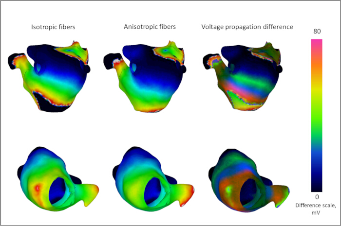
Figure 11. Verification of tissue anisotropy effects on action potential propagation. Comparison of transmembrane voltage maps during sinus rhythm simulation for the representative model using uniform isotropic fiber orientations (left column) and the reconstructed linearly interpolated transmural fiber field (middle column). The right column shows the absolute difference in voltage propagation between the two models. The color scale indicates the transmembrane voltage difference in millivolts (mV), ranging from 0 – 80 mV. Regions exhibiting high voltage differences highlight areas where directional fiber guidance is most critical, demonstrating how the anatomically reconstructed model eliminates wavefront discontinuities characteristic of uniform isotropic models. Please click here to view a larger version of this figure.

Resultaten

Validation of fiber orientation transfer and possible spatial errors

Figure 3 shows the quantitative assessment of the sensitivity of fiber transfer to the positions of auxiliary points for the representative model. The Root Mean Square Deviation (σ, RMSD) of the fiber direction components along each coordinate axis was computed at every surface point and visualized as a scalar field. Angular deviations were derived from the absolute component-wise deviations. Under broad landmark placement, the mean RMSD angular deviation for the reference model was 5.9° for the epicardium and 3.1° for the endocardium; with careful placement near optimal positions, these values were reduced to 0.6° and 1.1°, respectively. Across all 6 models, under broad landmark placement, the mean RMSD angular deviation was 4.1 ± 0.8°; with careful placement near optimal positions, this was reduced to 1.0 ± 0.4°. Furthermore, the surface area exhibiting non-zero variance (σ > 0) decreased substantially, from 32% to 10% of the epicardial surface and from 26% to 7% of the endocardial surface. In the constrained-placement scenario, regions of elevated variance were predominantly localized near the pulmonary vein ostia and the appendage. When auxiliary landmarks were selected within a reasonable neighborhood of 5 mm from their anatomically appropriate positions, deviations in the resulting fiber field were localized to regions of the myocardium, and the magnitude of directional error remained around 1° on average.

Thus, while strict adherence to anatomical guidelines minimized average deviations to 1°, residual errors persisted locally, primarily affecting the pulmonary vein ostia and the left atrial appendage, with occasional error peaks reaching 15–20°.

Figure 8 compares fiber orientations transferred from the atlas to the patient-specific atrial geometry using the UAC framework with those obtained via diffeomorphic deformation for the representative model. Although both methods yielded predominantly aligned fiber fields, measurable angular deviations (θ) were present. This angle served as a quantitative metric for assessing the fidelity of the transfer process in accommodating patient-specific morphological variability. Figures 8A, B display the spatial distribution of the angular transfer error θ for the epicardial and endocardial layers, respectively. The accompanying histograms illustrate the distribution of mean fiber transfer errors across all mesh elements, ranging from 0° to 80°. Analysis of angular deviations demonstrated alignment metrics. Specifically, for the 0–80° deviation distribution, the median error (50th percentile) was 28.9° for the epicardial layer and 29.4° for the endocardial layer. Color-coded maps revealed that deviations were predominantly localized to the posterior wall in the epicardium and the anterior wall in the endocardium. This spatial pattern likely reflects the inherent topological constraints of the UAC system, which requires surface incisions to partition the anterior and posterior domains during coordinate construction.

Although UAC-based mapping effectively preserved the dominant atrial fiber architecture, localized inaccuracies in fiber transfer occurred, particularly in anatomically complex regions such as the pulmonary vein ostia, the mitral valve annulus, and the left atrial appendage.

Transmural fiber interpolation and anatomical continuity

Figures 9A, B provide a qualitative visual comparison of two methodologies for reconstructing intramural fiber architecture: threshold-based (step-wise) and linear interpolation. The threshold-based approach assigns a discrete, layer-specific direction, resulting in an abrupt change in fiber orientation at the transmural midpoint (γ = 0.5). This produces distinctly segmented fields with sharp boundaries between opposing layers and abrupt transitions at intra-layer junctions. In contrast, linear interpolation generates a smooth, fan-like transition of fiber orientations from the epicardium to the endocardium. This yields a continuous rotational gradient in which vectors gradually transition across the wall thickness. These methodological differences are most visually pronounced in the color maps of regions where epicardial and endocardial fibers are nearly orthogonal, highlighted in blue and red.

To evaluate how these distinct fiber architectures influence wavefront propagation, a quantitative analysis of fiber angular deviations and Local Activation Times (LATs) was subsequently performed.

Figure 10A shows the differences in fiber orientation between threshold-based and linear interpolation methods for the representative atrial model. Differences were assessed by calculating the angular deviation in fiber direction at each point within the atrial myocardium. Results for all other reconstructed models are provided in Supplementary File 1 Section 4. Directional differences were quantified as angular deviations ranging from 0° to 90°. For the representative model, the mean angular deviation between threshold-based and linear interpolation methods was 7.89 ± 1.08°. Across all six cases, the mean angular deviation between threshold-based and linear interpolation methods was 8.06 ± 1.13°, indicating relatively good agreement between methods in most regions.

However, maximum angular deviations approaching 90° were observed primarily in the mid-myocardial region, where the epicardial and endocardial fiber layers converge in the case of threshold interpolation. Additionally, notable differences accumulated in several anatomically complex regions, including the atrial appendage and adjacent areas of the anterior and posterior atrial walls, designated as Region 1; the regions surrounding the pulmonary vein ostia; and the anterior wall region near the mitral valve, designated as Region 2. Regions 1 and 2 are indicated by dashed lines in Figure 10B. The maximum angular deviation in these regions reached 60° among all models. For the representative model, the average angular deviation was 38 ± 14° in Region 1 and 28 ± 15° in Region 2.

The effect of these interpolation differences on excitation wave propagation, particularly local activation time, varied in magnitude and was therefore investigated further in the subsequent section.

Electrophysiological propagation dynamics

Figure 11 presents action potential propagation maps for the patient-specific atrial model, comparing simulations with isotropic fiber orientations in the left column and interpolated transmural fibers in the middle column, thereby verifying the functional presence of tissue anisotropy. The resulting discrepancies in wavefront morphology highlight regions where directional fiber guidance most strongly influences simulated propagation. Anisotropic conduction effects are particularly evident around the pulmonary veins and the left atrial appendage, where the reconstructed model demonstrates anisotropy-directed wavefront propagation. Conversely, near the mitral valve annulus, the uniform isotropic model produces artificial wavefront breaks and fragmentation, which are eliminated when the anatomically reconstructed anisotropic fiber field is applied. This comparison demonstrates that the proposed mapping strategy incorporates directional fiber-dependent anisotropy into the computational model, particularly in zones of high geometric complexity.

Figure 10B shows the results of the quantitative analysis conducted to assess whether the choice of transmural fiber interpolation method has a measurable and statistically significant effect on macroscopic wavefront propagation and local activation patterns.

To quantify this tissue-level impact, two distinct fiber configurations were compared across six patient-specific computational models of the left atrium: threshold-based interpolation and linear interpolation. Electrophysiological simulations were performed using a monodomain formulation with the Courtemanche model and a pacing protocol applied at the left atrial roof with progressively decreasing cycle lengths. The mean conduction velocity for the representative model was 70 ± 2 cm/s for the threshold-based fibers and 71 ± 3 cm/s for the linearly interpolated fibers. The basic cycle length for the model was 72 ± 1 ms.

Local Activation Times (LATs) were specifically evaluated in two regions of interest that exhibited maximal transmural fiber divergence across all models: the lateral wall near the left pulmonary veins and left atrial appendage (Region 1), and the anterior wall adjacent to the mitral valve (Region 2). These regions were defined previously in the Transmural Fiber Interpolation section. Spatial maps detailing LAT differences for the other individual models are provided in Supplementary File 1 Section 4.

Statistical analysis revealed that the interpolation method systematically altered activation timing in these regions. In Region 1, the mean LAT difference between the two methods was 2.0 ± 0.6 ms, with the Wilcoxon signed-rank test confirming that linear interpolation systematically delayed activation compared with the threshold-based method (p = 0.031). Conversely, in Region 2, the threshold-based method delayed activation by a mean of −1.3 ± 0.5 ms compared with linear interpolation, which was also statistically significant (p = 0.031). Given that the basic cycle length across all atrial models was 75 ± 4 ms, this variation corresponded to 6.1 ± 1.5%.

Figure 12 provides a comprehensive overview across the entire cohort. It includes a summary diagram presenting LATs averaged across all six patient-specific models for both fiber configurations in the two regions of interest. For all numerical values, see Supplementary Table 1.

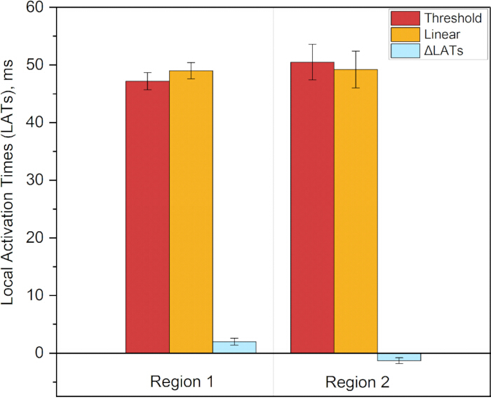
Figure 12. Local Activation Times (LATs) across all six patient-specific models for both fiber configurations in the two regions of interest. The first data series shows the average LAT across all models with threshold-based fiber interpolation, and the second shows the average LAT across all models with linear transmural interpolation. The ΔLAT series shows the average change in LAT between the two methods for each region: ΔLAT₁ = 2.0 ± 0.6 ms (p = 0.031) and ΔLAT₂ = −1.3 ± 0.5 ms (p = 0.031). Please click here to view a larger version of this figure.

Supplementary File 1: Additional methodological details and analyses supporting the patient-specific atrial fiber reconstruction pipeline. The file contains Supplementary Section 1, describing the cardiac segmentation protocol from CT data; Supplementary Section 2, describing the sensitivity analysis of auxiliary landmark placement; Supplementary Section 3, providing the detailed mathematical formulation of fiber vector transformation; and Supplementary Section 4, presenting additional analyses of the effects of transmural fiber interpolation methods on atrial electrophysiology. Please click here to download this file.

Supplementary Figure 1: Visualization of a CT scan in the 3D Slicer program. The central and bottom panels present axial, sagittal, and coronal CT views with manually placed seed markers, shown as colored regions, corresponding to each anatomical structure.Please click here to download this file.

Supplementary Figure 2: Manual annotation of anatomical seed regions in 3D Slicer for semi-automatic cardiac chamber segmentation. The left panel displays the segmentation module with the list of target cardiac structures: Left Atrium (green), Left Ventricle (red), Right Ventricle (blue), Right Atrium (cyan), Aorta (dark green), Pulmonary Artery (purple), and Vena Cava (orange). The central and bottom panels present axial, sagittal, and coronal CT views with manually placed seed markers corresponding to each anatomical structure. The upper-right panel shows a 3D volumetric view illustrating the spatial distribution of the annotated seed regions across the cardiac geometry. These labeled seeds serve as the initial input for the “Grow from Seeds” region-growing algorithm to automatically delineate the boundaries of each cardiac chamber and great vessel from the high-resolution CT volume.Please click here to download this file.

Supplementary Figure 3: Resulting whole-heart segmentation after automated segmentation using the “Grow from Seeds” tool. The figure shows the resulting whole-heart segmentation obtained after application of the automated segmentation procedure.Please click here to download this file.

Supplementary Figure 4: Preprocessing and surface regularization of the patient-specific left atrium segmentation. (A) Initial 3D surface mesh derived from clinical CT imaging, displaying raw vascular extensions, topological noise, and surface irregularities. (B) Finalized watertight geometric model after removal of extraneous vascular stubs and application of surface smoothing algorithms.Please click here to download this file.

Supplementary Figure 5: Blood pool and atrial wall segmentation. (A) Initial 3D surface reconstruction before topological cleaning, showing the raw segmented geometry, including residual blood pool structures and surface artifacts. (B) Resulting atrial wall model after topological cleaning and artifact removal, yielding a continuous watertight surface mesh ready for volumetric finite-element generation.Please click here to download this file.

Supplementary Figure 6: Finalized patient-specific geometric models of the left atrium. (A) Reconstructed epicardial surface mesh representing the outer boundary of the atrial myocardium. (B) Reconstructed endocardial surface mesh representing the inner boundary adjacent to the blood pool. (C) Resulting atrial wall geometry integrating both surfaces to define the myocardial thickness required for the derivation of the continuous transmural coordinate and subsequent volumetric fiber mapping.Please click here to download this file.

Supplementary Figure 7: Example of application of the pipeline to MRI data from the AtriaSeg 2018 Challenge dataset. (A) Use of a pre-existing atrial wall and blood pool segmentation from the AtriaSeg 2018 Challenge dataset to create a 3D atrial model according to Protocol Section 1. (B) Marking of the veins and atrial appendage for the epicardial and endocardial layers according to Protocol Section 2. (C) Unfolding of the epicardial and endocardial 3D models into a two-dimensional atrial coordinate system, 2D UAC, according to Protocol Section 3. (D) Introduction of the transmural coordinate γ and creation of the 3D UAC system according to Protocol Section 4. (E) Resulting 3D atrial model with transmural fibers.Please click here to download this file.

Supplementary Figure 8: Selection of points for sensitivity assessment. The optimal positions of the points selected in Protocol Section 2.1 are shown in white. Red indicates positions selected within a broad range from the reference point (<15 mm). Green indicates positions selected within a limited range from the reference point (<5 mm).Please click here to download this file.

Supplementary Figure 9: Sensitivity analysis of fiber orientation transfer to auxiliary landmark placement variability. The color maps represent fiber variance magnitude in arbitrary units. σ_angle max denotes the maximum standard deviation of the angle for a given atrial model, and σ_angle average denotes the average value of the deviation angles. Upper row: Epicardial surface. Under broad landmark placement, σ_angle max reaches 31.6°, with σ_angle average of 4.6°. When landmarks are constrained to their optimal anatomical neighborhood, σ_angle max decreases to 18.5° and σ_angle average decreases to 1.4°. Lower row: Endocardial surface. Under broad landmark placement, σ_angle max is 32.7°, with σ_angle average of 3.8°. With constrained landmark placement, σ_angle max decreases to 14.8° and σ_angle average decreases to 0.9°.Please click here to download this file.

Supplementary Figure 10: Sensitivity analysis of fiber orientation transfer to auxiliary landmark placement variability. The color maps represent fiber variance magnitude in arbitrary units. σ_angle max denotes the maximum standard deviation of the angle for a given atrial model, and σ_angle average denotes the average value of the deviation angles. Upper row: Epicardial surface. Under broad landmark placement, σ_angle max reaches 32.8°, with σ_angle average of 4.1°. When landmarks are constrained to their optimal anatomical neighborhood, σ_angle max decreases to 19.0° and σ_angle average decreases to 1.1°. Lower row: Endocardial surface. Under broad landmark placement, σ_angle max is 28.7°, with σ_angle average of 3.6°. With constrained landmark placement, σ_angle max decreases to 13.8° and σ_angle average decreases to 0.9°.Please click here to download this file.

Supplementary Figure 11: Sensitivity analysis of fiber orientation transfer to auxiliary landmark placement variability. The color maps represent fiber variance magnitude in arbitrary units. σ_angle max denotes the maximum standard deviation of the angle for a given atrial model, and σ_angle average denotes the average value of the deviation angles. Upper row: Epicardial surface. Under broad landmark placement, σ_angle max reaches 33.0°, with σ_angle average of 3.2°. When landmarks are constrained to their optimal anatomical neighborhood, σ_angle max decreases to 22.0° and σ_angle average decreases to 1.4°. Lower row: Endocardial surface. Under broad landmark placement, σ_angle max is 54.3°, with σ_angle average of 4.6°. With constrained landmark placement, σ_angle max decreases to 21.8° and σ_angle average decreases to 1.5°.Please click here to download this file.

Supplementary Figure 12: Sensitivity analysis of fiber orientation transfer to auxiliary landmark placement variability. The color maps represent the magnitude of fiber variance in arbitrary units. σ_angle max denotes the maximum standard deviation of the angle for a given atrial model, and σ_angle average denotes the average value of the deviation angles. Upper row: Epicardial surface. Under broad landmark placement, σ_angle max reaches 27.5°, with σ_angle average of 4.3°. When landmarks are constrained to their optimal anatomical neighborhood, σ_angle max decreases to 20.5° and σ_angle average decreases to 0.9°. Lower row: Endocardial surface. Under broad landmark placement, σ_angle max is 37.1°, with σ_angle average of 4.4°. With constrained landmark placement, σ_angle max decreases to 16.0° and σ_angle average decreases to 0.8°.Please click here to download this file.

Supplementary Figure 13: Sensitivity analysis of fiber orientation transfer to auxiliary landmark placement variability. The color maps represent the magnitude of fiber variance in arbitrary units. σ_angle max denotes the maximum standard deviation of the angle for a given atrial model, and σ_angle average denotes the average value of the deviation angles. Upper row: Epicardial surface. Under broad landmark placement, σ_angle max reaches 33.0°, with σ_angle average of 5.0°. When landmarks are constrained to their optimal anatomical neighborhood, σ_angle max decreases to 15.2° and σ_angle average decreases to 1.1°. Lower row: Endocardial surface. Under broad landmark placement, σ_angle max is 52.5°, with σ_angle average of 3.7°. With constrained landmark placement, σ_angle max decreases to 14.0° and σ_angle average decreases to 1.0°.Please click here to download this file.

Supplementary Figure 14: Scheme of the fiber transfer process from the atlas to the patient-specific atrial model. Element centroids of the target mesh, expressed in Universal Atrial Coordinates (UAC), are spatially registered to the atlas UAC grid using a nearest-neighbor search (KD-tree, k = 1) for each anatomical region. Consequently, every element of the patient-specific mesh is assigned the fiber orientation corresponding to its nearest atlas counterpart.Please click here to download this file.

Supplementary Figure 15: Fiber orientation estimation by visual comparison of reconstructed fiber orientations with the deformed atlas atrium. Atlas-derived fiber orientations are shown in red, and reconstructed fiber orientations are shown in cyan. The overlay illustrates the correspondence between the atlas-derived and reconstructed fiber orientations in the patient-specific atrium.Please click here to download this file.

Supplementary Figure 16: Quantitative comparison of transmural fiber interpolation methods and their functional impact on atrial electrophysiology. (A) Spatial distribution of angular deviations in fiber orientation between threshold-based and linear interpolation methods. Angular deviations were calculated at each point within the atrial myocardium and ranged from 0° to 90°. (B) Quantitative assessment of Local Activation Time (LAT) differences between threshold-based and linear interpolation methods. LATs were evaluated across the whole model.Please click here to download this file.

Supplementary Figure 17: Quantitative comparison of transmural fiber interpolation methods and their functional impact on atrial electrophysiology. (A) Spatial distribution of angular deviations in fiber orientation between threshold-based and linear interpolation methods. Angular deviations were calculated at each point within the atrial myocardium and ranged from 0° to 90°. (B) Quantitative assessment of Local Activation Time (LAT) differences between threshold-based and linear interpolation methods. LATs were evaluated across the whole model.Please click here to download this file.

Supplementary Figure 18: Quantitative comparison of transmural fiber interpolation methods and their functional impact on atrial electrophysiology. (A) Spatial distribution of angular deviations in fiber orientation between threshold-based and linear interpolation methods. Angular deviations were calculated at each point within the atrial myocardium and ranged from 0° to 90°. (B) Quantitative assessment of Local Activation Time (LAT) differences between threshold-based and linear interpolation methods. LATs were evaluated across the whole model.Please click here to download this file.

Supplementary Figure 19: Quantitative comparison of transmural fiber interpolation methods and their functional impact on atrial electrophysiology. (A) Spatial distribution of angular deviations in fiber orientation between threshold-based and linear interpolation methods. Angular deviations were calculated at each point within the atrial myocardium and ranged from 0° to 90°. (B) Quantitative assessment of Local Activation Time (LAT) differences between threshold-based and linear interpolation methods. LATs were evaluated across the whole model.Please click here to download this file.

Supplementary Figure 20: Quantitative comparison of transmural fiber interpolation methods and their functional impact on atrial electrophysiology. (A) Spatial distribution of angular deviations in fiber orientation between threshold-based and linear interpolation methods. Angular deviations were calculated at each point within the atrial myocardium and ranged from 0° to 90°. (B) Quantitative assessment of Local Activation Time (LAT) differences between threshold-based and linear interpolation methods. LATs were evaluated across the whole model.Please click here to download this file.

Supplementary Table 1: Local Activation Times (LATs) across all six patient-specific models for both transmural fiber interpolation methods in two regions of interest. Region 1 corresponds to the lateral wall near the left pulmonary veins and left atrial appendage. Region 2 corresponds to the anterior wall adjacent to the mitral valve. LATs_threshold represents Local Activation Times obtained with threshold-based (step-wise) transmural fiber interpolation, and LATs_linear represents Local Activation Times obtained with continuous linear transmural fiber interpolation. ΔLAT represents the difference in Local Activation Times between the two interpolation methods. All values are presented in milliseconds (ms). Mean and standard deviation (SD) are calculated across all six patient-specific models.Please click here to download this file.

Discussie

The present study introduces and validates a comprehensive, open-source pipeline for patient-specific atrial fiber orientation mapping using a 3D extension of the Universal Atrial Coordinate (UAC) framework. By releasing the fully open-source processing pipeline, the study also makes the underlying computational assets publicly available, including high-resolution CT volumes, segmentations, and patient-specific finite-element meshes ready for electrophysiological studies. By systematically evaluating the methodology from geometric reconstruction to functional electrophysiological outcomes, this work provides critical insights into the role of transmural fiber interpolation in computational cardiac modeling.

The robustness of the UAC framework relies on several critical steps. First, accurate identification of auxiliary anatomical landmarks for surface parametrization is paramount. The sensitivity analysis demonstrated that, while the method is highly robust, landmark placement must adhere to a strict anatomical neighborhood, approximately 5 mm from optimal positions. Deviations beyond this threshold, particularly in the placement of points defining anterior/posterior wall separation, can induce localized angular error spikes reaching 15–20°. Troubleshooting such deviations requires strict adherence to the provided anatomical guidelines, with a focus on stable landmarks such as the pulmonary vein ostia and the appendage base. Second, the derivation of the continuous transmural coordinate γ via the Laplace–Dirichlet problem is a mathematically rigorous step that ensures topological consistency across the thin atrial wall and avoids artifacts associated with simple distance-based metrics.

Beyond transmural coordinate derivation, the accuracy of transferring surface fiber orientations from the reference atlas to the patient-specific epicardial and endocardial geometries was rigorously evaluated. The mean angular transfer errors for the reconstructed atrial models were quantified as 28.9°–29.4°. While this range is higher than previously reported ventricular mapping errors, typically 15.4°–18.8°, this discrepancy is anatomically and biophysically expected. The primary driver of the elevated angular error in the atria is the substantial difference in wall thickness and the resulting spatial gradients of fiber rotation. The ventricular wall is relatively thick, 10–15 mm, allowing transmural fiber rotation, typically from −60° to +60°, to occur gradually over a large physical distance²⁹. In contrast, high-resolution DT-MRI studies demonstrate that the atrial wall is exceptionally thin, with an average thickness of 2.7 mm and a range of 1–4 mm, and exhibits highly heterogeneous fiber rotations of up to 60°–90°, depending on the region¹⁰. Atlas-based and rule-based mapping methods inherently struggle with such steep spatial gradients. When the underlying fiber orientation changes abruptly over a distance of merely 1–2 mm, any minor spatial misregistration or interpolation step inevitably results in a larger angular deviation. Therefore, an average surface transfer error of 29° in the atria is mathematically consistent with the much steeper transmural gradients, contrasting with the 6° error observed in the thicker, more gradually rotating ventricles.

While previous foundational studies have established the general utility of atlas-based mapping over generic rule-based methods, this work isolates and rigorously evaluates the transmural interpolation strategy itself. The qualitative and quantitative comparisons reveal that linear interpolation and threshold-based, step-wise methods represent fundamentally different mathematical assumptions regarding transmural fiber transition. Linear interpolation generates a smooth, continuous rotational gradient, whereas the threshold-based approach assigns discrete, layer-specific directions with abrupt mid-wall transitions. Rather than asserting the absolute superiority of one method, the study highlights that these distinct mathematical formulations yield measurably different intramural microstructures, particularly in regions with steep spatial gradients. Given that the true in vivo fiber architecture likely represents a complex, region-specific combination of both strategies, systematic comparison allows interpolation error to be bounded relative to the unknown ground truth.

A primary objective of this study was to evaluate how these distinct fiber transfer and interpolation choices affect the functional propagation of excitation waves. The comparison between isotropic and anatomically reconstructed models confirmed that the UAC pipeline effectively imparts physiological anisotropy, resolving artificial wavefront breaks and fragmentation, for example, near the mitral valve annulus, that are characteristic of uniform models. More importantly, quantitative analysis of Local Activation Times (LATs) demonstrated that the choice of transmural interpolation is a functionally significant variable. The distinct mathematical assumptions of the interpolation methods systematically altered activation timing in anatomically complex zones, inducing statistically significant absolute LAT shifts of 1–3 ms (p = 0.031), with both increases and decreases observed. Given that the basic cycle length (BCL) across all atrial models ranged from 70 – 80 ms, the observed LAT variations of 5.0 ± 0.8 ms corresponded to 6.1 ± 1.5% of the pacing cycle, representing a physiologically meaningful proportion of the cardiac cycle duration. Given baseline atrial conduction velocities of 70–75 cm/s, these localized timing differences over short distances of 10–20 mm corresponded to conduction velocity changes of approximately 5%–10%. In the context of atrial electrophysiology, such alterations represent a measurable shift that can influence wavefront propagation dynamics and confirm that the choice of transmural fiber interpolation significantly affects local activation patterns in regions of maximal fiber divergence.

Several limitations must be acknowledged. First, the segmentation, mesh generation, and fiber mapping pipeline were developed and validated exclusively on high-resolution cardiac CT datasets with voxel dimensions of 0.4 × 0.4 × 0.625 mm³. The accuracy of the reconstructed fiber fields, particularly in regions of thin atrial wall and abrupt transmural transitions, is inherently tied to this spatial resolution. While the underlying mathematical framework of the UAC system is modality-agnostic and can be applied to both CT and MRI data, the rigorous quantitative validation, error bounding, and electrophysiological simulations presented in this study were derived exclusively from high-resolution CT datasets with voxel dimensions of 0.4 × 0.4 × 0.625 mm³. Generalizability to lower-resolution clinical MRI with typical voxel sizes of 1.25 × 1.25 × 2.5 mm³ requires further dedicated evaluation and may be affected by partial volume effects and reduced boundary definition.

Additionally, the electrophysiological simulations were performed using a single-monodomain formulation coupled to the Courtemanche-Ramirez-Nattel human atrial cell model. Given the exceptionally thin atrial wall of 1–3 mm, the choice of tissue-level model, including monodomain versus bidomain formulations, boundary conditions at tissue-blood interfaces, and cellular ionic model, may influence the absolute values of conduction velocity and activation times. However, the primary objective of this computational study was not to predict absolute activation sequences with clinical precision, but rather to quantitatively assess the relative differences in Local Activation Times induced by different transmural fiber interpolation strategies.

Finally, while the sensitivity of the model to varying pacing cycle lengths of 200–300 ms was evaluated, the tissue-level conductivity tensor ratio, with longitudinal conductivity (σ_L) to transverse conductivity (σ_T) fixed at 4:1, using σ_L = 0.4 S/m and σ_T = 0.1 S/m, was held constant across all simulations. This ratio represents the standard consensus value for human atrial tissue in computational electrophysiology¹⁸˒²². Varying this ratio would require patient-specific tissue characterization, for example, fibrosis mapping using LGE-MRI, which is beyond the CT-based anatomical modeling. Future studies may integrate multimodal imaging to explore the sensitivity of interpolation effects to spatially varying degrees of bulk tissue anisotropy under different pathophysiological conditions.

The broader value of this work extends beyond methodological validation to the advancement of open science in cardiac modeling. By releasing the fully open-source processing pipeline alongside high-resolution, patient-specific CT-based atrial models, this study provides a robust and accessible resource for the broader research community. For research groups lacking direct access to patient-specific DT-MRI data or specialized fiber-mapping algorithms, this openly shared framework offers a mathematically rigorous alternative to simplistic, uniform fiber assumptions.

Open-source pipelines that implement diverse approximation strategies for myocardial microstructure, derived from clinically accessible preoperative imaging, may support the future development of recommendation systems for targeted ablation planning. By systematically comparing different interpolation methods and quantifying their inherent errors, these frameworks may complement mechanistic computational predictions with a rigorous assessment of model reliability. Ultimately, integrating this quantification of uncertainty is a critical prerequisite for safely translating in silico simulations into clinical decision-making.

Materialen

Lijst van materialen gebruikt in dit artikel

Naam	Bedrijf	Catalogusnummer	Opmerkingen
3D Slicer	Open-source	v5.8.1; https://www.slicer.org/	Open-source medical image computing platform used for CT visualization, segmentation, surface extraction, and preparation of atrial geometries.
Computed tomography (CT) data	City Clinical Hospital named after I.V. Davydovsky	N/A; https://zenodo.org/records/21855641	Patient-specific cardiac CT datasets used for atrial reconstruction, including segmented epicardial and endocardial surfaces and reconstructed atrial wall models. The cohort comprised 6 patients (5 males, 1 female; age 57–66 years) with persistent atrial fibrillation lasting ≥3 years.
Custom processing pipeline code	Moscow Center for Advanced Studies	N/A; https://github.com/AnastasiyaSinitsyna/transmural_atrial_fiber_mapping.git	Custom scripts and processing code used to reproduce the atrial geometry, coordinate mapping, fiber transfer, transmural interpolation, and analysis workflow described in the protocol.
Human Atrial Fibre Atlas	Johns Hopkins University / Open-source	N/A; https://zenodo.org/records/3764917	Reference atrial fiber atlas used for transfer of epicardial and endocardial fiber orientations to patient-specific geometries.
Meshalyzer	Open-source	v6.2; https://git.opencarp.org/openCARP/meshalyzer/-/releases	Scientific visualization software used to inspect cardiac meshes, fiber orientations, and electrophysiological simulation outputs.
Meshtool	Open-source	v1.0; https://bitbucket.org/aneic/meshtool/src/master/	Mesh-processing utility used for conversion, manipulation, and preparation of cardiac meshes for downstream openCARP simulations.
NVIDIA Tesla K20 GPU	NVIDIA	N/A	Graphics processing unit used with a 32-core CPU for parallel electrophysiological simulations. Under this hardware configuration, approximately 1 h of computation time was required to simulate 10 s of electrophysiological activity.
openCARP	Open-source	v12; https://opencarp.org/	Open-source cardiac electrophysiology simulation environment used to perform monodomain simulations and evaluate local activation times and wavefront propagation.
ParaView	Open-source	v6.0.0; https://www.paraview.org/	Open-source scientific visualization software used for inspection and quality assessment of reconstructed geometries, meshes, and fiber fields.