Feature Extraction from Space Debris Point Clouds with Geometry-Guided Contour Extraction and Multilayer Perceptron

Samenvatting

Space Debris Point Cloud Feature Extraction Network (SFENet) combines geometry-guided contour extraction with a multilayer perceptron for space-debris point-cloud feature extraction. The method identifies contour candidates from local point distributions and learns discriminative feature representations for classification. Experiments on SpaceSense-Bench demonstrate effective feature classification and contour extraction under the evaluated simulation conditions.

Samenvatting

Feature extraction of space debris from point cloud data faces challenges such as difficulty in contour extraction, structural complexity, and strong noise interference. To address these challenges, we propose the Space Debris Point Cloud Feature Extraction Network (SFENet), which combines geometry-guided contour extraction with a multilayer perceptron (MLP). First, a geometry-guided contour extraction procedure analyzes local neighborhoods of the three-dimensional point cloud. Spherical neighborhoods are divided into angular sectors, and the distribution of neighboring points is evaluated to identify sparse or empty regions associated with candidate contour points. The resulting contour candidates are then processed by the MLP-based feature learning network to obtain discriminative local and global representations. Second, in the feature learning stage, a multilayer perceptron network is constructed. Through hierarchical abstraction and multi-scale feature fusion, the point cloud is effectively extracted. Finally, multiview point cloud registration and classification experiments are conducted to evaluate the geometric quality, robustness, and feature representation capability of the proposed framework. Experimental results show that SFENet achieves an RMSE of 0.173 cm in the post-hoc contour reconstruction evaluation and effectively classifies multi-class features under simulated conditions. These results on the SpaceSense-Bench simulation dataset show that SFENet provides effective feature representation and accurate contour candidates under the evaluated simulation conditions. These results demonstrate the potential of the proposed framework for downstream space-debris perception and geometric reconstruction, while further validation using real sensor measurements is required to establish its robustness in practical on-orbit environments.

Inleiding

Space debris in space varies in shape, structure, and type. Traveling at high speeds in orbit, even small debris can cause catastrophic consequences upon collision with a spacecraft¹. Debris larger than 1 cm is sufficient to cause serious damage, while millimeter- or even micrometer-sized debris can degrade spacecraft performance or even cause malfunctions. For space debris larger than 10 cm, active removal technology is necessary, and the first step in this process is capture². The choice of capture method depends on factors such as the size and structural characteristics of the space debris, as well as the debris's volume relative to the capture system. Therefore, to effectively capture different types of space debris, it is necessary to systematically classify and summarize their shape and structural characteristics³. This will enable space mechanical capture mechanisms to adopt appropriate capture strategies for different types of debris, improving mission success rates and adaptability.

Currently, non-contact measurement is the primary method for close-range measurement of space debris⁴. Studies have proposed using line segment detectors to extract linear features from targets, while others combine background segmentation with morphological processing for three-dimensional (3D) image reconstruction based on Inverse Synthetic Aperture Radar (ISAR)⁵, measuring the size of rectangles by identifying their long and short sides. For the triangular support structures commonly found in decommissioned satellites, a triangular feature recognition method based on binocular vision and least-squares matching (LSM)⁶ has been proposed. Furthermore, for circular nozzle structures in spacecraft, studies have also achieved effective detection of circular features based on least-squares matching⁷.

Compared to two-dimensional images, point cloud data⁸ can more directly and accurately reflect the geometric structure and spatial distribution characteristics of three-dimensional targets, thus having a significant advantage in space target shape analysis⁹. With the continuous development and deep integration of radar and aerospace technologies, modern spacecraft are typically equipped with high-performance radar equipment, enabling active detection of space targets in orbit and direct acquisition of three-dimensional point cloud data describing their shape and structure. Compared to traditional imaging methods, point cloud data is less affected by lighting conditions during acquisition and can provide richer spatial geometric information, thus gradually becoming an efficient and reliable means of acquiring the shape characteristics of space debris¹⁰.

Existing methods for point cloud contour extraction can be broadly categorized into two types: one projects the 3D point cloud onto a 2D plane and performs boundary detection using image processing techniques¹¹. This method is simple to implement and computationally efficient, but inevitably suffers from spatial information loss during projection, affecting detection accuracy. The other type directly analyzes the geometric features of the point cloud, such as using neighborhood normals, curvature variations, and gradient information for contour recognition¹². This method makes fuller use of 3D structural information and typically achieves higher accuracy, but it is computationally complex.

To further improve the robustness and generalization ability of algorithms, researchers have recently begun to introduce deep learning methods for point cloud contour detection. These methods, by constructing neural network models, can automatically learn complex spatial feature representations and exhibit greater adaptability to noise, missing data, and shape diversity. However, due to the complex structural forms of space debris and limited prior information, deep learning models often rely on large amounts of labeled data for training. This not only increases the cost of data acquisition and labeling but also places higher demands on computational resources and processing speed, posing certain challenges in practical applications. Motivated by the limitations of existing approaches, this paper proposes a Space Debris Point Cloud Feature Extraction Network (SFENet) that combines geometry-guided contour extraction¹³ with a Multilayer Perceptron (MLP)¹⁴. SFENet combines geometric priors and feature learning to improve contour extraction and reconstruction performance for space debris point clouds. SFENet consists of two complementary components. The geometry-guided contour extraction (GCE) module extracts contour candidates using local spherical neighborhoods and eight-sector azimuthal point-distribution analysis, while the MLP-based feature network learns discriminative local and global representations from the extracted contour information. The overall performance improvement results from the interaction of geometry-guided contour localization and data-driven feature learning. There are three contributions of this work as follows.

1. A geometry-guided contour extraction method is developed for three-dimensional space debris point clouds. The method analyzes local point distributions within spherical neighborhoods and angular sectors to identify candidate contour points. The extracted candidates provide geometrically meaningful inputs for subsequent contour reconstruction and registration evaluation.
2. The feature extraction network, which consists of an SA layer, a feature extraction layer, and a feature processing layer, uses the recognition accuracy of point cloud objects as the driving force for network parameter updates.
3. The MLP learns discriminative feature representations from the geometry-guided contour information and performs object classification, while contour reconstruction and multi-view registration are conducted as downstream evaluations of the extracted features.

The primary objective of this work is feature extraction for space debris point clouds and object classification. The quality of the extracted geometric information is further evaluated through contour reconstruction and multi-view registration. To achieve robust feature representation, the proposed SFENet first performs geometry-guided sector-based contour extraction to identify contour-related points that preserve the geometric structure of the target. These contour points are then used as the input to the MLP-based feature learning network, which learns discriminative local and global representations for object classification. Multi-view registration and contour reconstruction are employed only as auxiliary evaluations to verify the geometric quality and robustness of the extracted contour features, rather than as independent learning objectives.

Related works:
Point cloud feature extraction technology
Generally, point cloud data can clearly depict the shape features of an object or environment. However, direct processing of point cloud data is time-consuming due to limitations in computing power, and the resulting object shape features are often blurry. Therefore, point cloud features are introduced to describe various shape features of objects or environments.

Evangelos et al.¹⁵ designed a robust skeleton extraction method specifically for accurately extracting curvature lines from point clouds. To reduce noise interference, robust statistical methods were first applied to estimate the surface's normal vector and curvature, and to eliminate isolated points. To accurately correct the data, the minimum energy method was used to ensure a more accurate and stable extracted skeleton. This method is applicable to various surfaces, retains sharp features, and is robust to noise and isolated points. Gunhold et al.¹⁶ proposed a feature extraction method. The algorithm calculates the average curvature of the point cloud, uses this curvature to fit a curve, and then classifies the fitted curves. Through further fitting processing, the feature line is finally obtained. Kalasi et al.¹⁷ designed the FALKO algorithm. The innovation of this algorithm is that it first identifies candidate points by analyzing the angles formed by edges between points in the neighborhood of the point. Then the algorithm divides the neighborhood of the candidate points in detail to more accurately describe their local geometric structure. Finally, the feature points are accurately extracted through the scoring mechanism. Zhang et al.¹⁸ proposed a statistical feature extraction method. In the neighborhood of a point cloud, the distance and normal angle between points are obtained through mathematical operations. When the angle exceeds the threshold, it is marked as a feature point, effectively distinguishing corner points from surface points while maintaining high accuracy and improving feature extraction efficiency.

Recent networks such as PointNet, PointNet++, and PointNeXt¹⁹ improved pointwise and multi-scale feature learning. Contour methods have shifted from curvature rules toward hybrid geometric-learning models. However, most approaches still separate contour localization from discriminative learning, leaving a gap in the joint preservation of contour structure and the extraction of robust space-debris features.

Conformal geometric algebra
In 1879, Clifford first proposed geometric algebra²⁰. In 2001, Li et al.²¹ proposed Conformal Geometric Algebra (CGA), also known as the generalized homogeneous coordinate system, which is a new geometric representation and computation system. As a combination of advanced geometric invariants and covariate systems, it provides a unified, concise, homogeneous algebraic representation of classical geometry. Its characteristic is that it can perform simplification operations such as expansion and elimination on complex symbolic geometric calculations in geometric algebra. More importantly, its geometric invariant properties are widely used in elementary geometry, especially in geometric calculations and data processing, where they offer significant advantages. CGA is widely used in other fields, such as remote sensing²², Robots²³, computer graphics²⁴, and aircraft^25,26. For example, Li et al.²⁷ proposed a novel algorithm for extracting the contour of a rolling target from space debris based on CGA. This algorithm maps 3D point cloud data from Euclidean space to conformal space and uses geometric relationships such as points, lines, and surfaces to uniformly represent candidate contour points, thereby extracting the complete target outline. This method combines multi-view stitching and concavity/convexity feature determination in conformal space, effectively reducing computational complexity and improving the speed and robustness of contour point extraction. Wu and Jiao²⁶ proposed a Flight Conflict Detection Algorithm (FCDA) based on Cylindrical Protection Zones (CPZ) using CGA to improve reaction time for air traffic controllers and pilots. By representing CPZs with CGA forms of the cylinder’s central circle and axis segments, and leveraging inner, outer, and geometric product operations, the algorithm efficiently determines positional relationships and detects potential flight conflicts.

Recent contour extraction and geometric representation approaches have increasingly incorporated learning-based strategies and geometry-aware feature modeling. Compared with traditional methods relying on curvature estimation or local neighborhood statistics, these approaches improve robustness under complex geometric structures and noisy environments. However, many existing methods either focus primarily on feature learning or geometric processing independently, making it difficult to simultaneously preserve contour structures and learn discriminative representations.

Multilayer perceptrons
Multilayer Perceptrons (MLPs)²⁸, as one of the most classic feedforward neural network models, have been widely used in feature extraction and representation learning. Traditional feature extraction methods often rely on hand-designed features or geometric descriptors, which tend to have limited performance in complex environments. MLPs, through layer-by-layer nonlinear transformations and weight learning, can automatically extract high-dimensional, abstract feature representations from raw data, thus significantly improving feature representation capabilities and task performance. In image processing and computer vision, MLPs are used to extract semantic features from pixel-level input for classification, object detection, and segmentation tasks²⁹. In 3D point cloud and spatial data processing, researchers use point cloud coordinates or local geometric descriptions as input to leverage MLPs to learn local and global features, thereby achieving tasks such as object recognition, pose estimation, and environment reconstruction³⁰.

In recent years, deep learning architectures combined with MLPs, such as PointNet³¹ and PointNet++, have further improved feature extraction capabilities. These methods encode point-by-point features in point clouds using multi-layer MLP modules and construct global feature representations using pooling operations. For instance, Zhang et al.³² proposed a novel multilayer perceptron (MLP) method for learning local features in point clouds, called L2MLP. This method comprises two key modules. First, applying an MLP (channel interaction module) to the feature channels of each point, and second, applying an MLP (point interaction module) to points within the local neighborhood, thus simultaneously emphasizing the interaction between channels and points. Compared to traditional methods, L2MLP can fully capture correlations among all points in the local neighborhood, yielding a more accurate local description while maintaining high computational efficiency due to its simple structure.

Protocol

To achieve high adaptability and multi-class capture of space debris, it is necessary to consider key physical properties, such as the target's shape and size, with accurate extraction of shape features being particularly crucial. For point cloud feature extraction, SFENet employs a multi-level network structure that learns local and global features of the point cloud layer by layer, thereby more effectively representing the complex geometric structure of space debris. Simultaneously, SFENet introduces a multi-scale grouping strategy to mitigate the impact of uneven point cloud distribution, enabling the model to fully capture structural information at different scales during feature extraction. Furthermore, SFENet optimizes its network structure and parameter configuration, improving computational efficiency while maintaining feature representation. SFENet can output fixed-dimensional feature representations and mainly consists of Set Abstraction layers, feature extraction layers, and feature processing layers, as shown in Figure 1.

The SFENet framework consists of two sequential stages: geometry-guided contour extraction and feature representation learning. First, GCE-based contour candidate extraction is applied to identify contour-related points by analyzing local spherical neighborhoods and eight-sector azimuthal occupancy. The resulting set of contour candidates is then used as input to the SA and MLP modules for hierarchical feature learning and classification. Therefore, the framework adopts a geometry-guided processing strategy rather than a fully end-to-end optimization architecture.

The overall processing pipeline consists of four stages. Input is raw three-dimensional point clouds of space debris. Stage 1 is GCE-based contour candidate extraction, which generates sets of contour-related points. Stage 2 is hierarchical MLP-based feature extraction that learns local and global geometric representations from the contour points. Stage 3 maps the extracted features to object categories via supervised classification with cross-entropy loss. The output consists of discriminative feature representations together with the predicted object category. Multi-view registration and contour reconstruction are subsequently performed only for performance evaluation and are not optimized during network training. The geometry-guided contour extraction strategy is motivated by the geometric representation principles of CGA, while the implemented procedure focuses on local spatial relationships and sector-based point distributions rather than explicit conformal algebraic operations.

Accordingly, the complete processing pipeline can be summarized as geometric contour localization, MLP feature learning, object classification, registration, and contour reconstruction. The first stage provides geometric contour candidates; the second stage learns discriminative representations; the third stage yields the primary classification output; and the final stage evaluates the geometric effectiveness of the extracted features via downstream registration and contour reconstruction.

3D Point cloud contour extraction

Unlike two-dimensional images, three-dimensional point clouds do not reflect information such as color, texture, and corner points. Instead, they reflect the appearance features that indicate the geometric structure of the point cloud model. These include point cloud density, noise points, principal curvature of individual points, and distances to neighboring points. Furthermore, the interaction of point cloud normals best reflects changes in the geometric features of the model's surface.

Principal component analysis (PCA)³³ is often used to estimate two-dimensional planes due to its dimensionality reduction principle. It requires selecting k-neighborhood points for each point and fitting these points into a plane using least-squares regression, as shown in Equation (1).

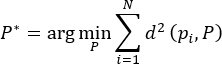(1)

Where p_i denotes the i-th point in the local point set, N is the number of points, and P denotes the parameters of the fitted plane. P* is the plane that minimizes the sum of squared point-to-plane distances d(p_i, P).

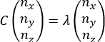
Let . The point Δp_i can be expressed in coordinates as . The covariance matrix C of the neighboring points satisfies Equation (2). Let λ be an eigenvalue of the covariance matrix C, and 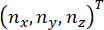 be the eigenvector corresponding to λ.

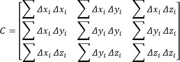(2)

(3)

The concavity or convexity of a region’s plane is represented by the angle θ_i between the normal vector of an arbitrary point and the normals of its k-nearest neighboring points. Flat regions have smaller normal angles, while areas with larger curvature changes have larger normal angles. Let d_i denote the distance between the point and its neighboring points. The distances between neighboring points serve as rotation-invariant features and also reflect the point cloud density. The value of d_i is obtained from the Euclidean distances between the current point and its neighbors. The relationship between them is expressed by Equation (4).

(4)

Where k is the number of neighboring points, is the Euclidean distance between the central point and its i-th neighbor p_i, and θ_i is the angle between their corresponding normal vectors.

The fitted plane is first obtained using Equation (1), and feature points are subsequently identified according to the distance-based threshold criterion defined in Equation (4). Then, a suitable threshold is selected. If , the point is considered a feature point and retained; otherwise, it is not a feature point.

The point cloud contour extraction algorithm consists of four steps: point cloud acquisition, candidate contour point extraction, multi-view registration, and final contour point determination. Identifying candidate contour points is a crucial step. Searching for contour points using KNN is effective, but it produces reprojected points and is very slow. Employing feature point extraction methods can preserve boundary information. Local spherical neighborhoods and eight azimuthal sectors are used to reduce computational complexity, thereby improving search speed. This paper proposes a geometry-guided sector-based algorithm, the pseudocode of which is shown in Algorithm 1. This algorithm processes a set of points (P) by examining the local neighborhood around each point to detect boundaries and guide exploration. For every point (p), a spherical region is constructed and divided into multiple angular sectors (m), and the distribution of neighboring points within each sector is computed as a probability measure. If one or more consecutive sectors contain no points, the current point is identified as a boundary point, and its neighbors contribute to the contour. Otherwise, the algorithm determines the sparsest sector and selects the farthest point in that direction to continue exploration. This process repeats iteratively until all points have been analyzed, enabling the detection of edges and the traversal of less dense regions in the dataset, and outputs boundary points (B) and a set of points forming the contour adjacent to boundary points (C). For the current point p, Ni denotes its local neighboring points within S(p,r), and Ns denotes the candidate points available for the subsequent search. NextPoint is selected as the farthest unvisited candidate point in the direction of the sector with the lowest point-distribution ratio. A visited point is excluded from subsequent selection. The iterative search terminates when no eligible unvisited candidate point remains. The spherical neighborhood centered at p is projected onto the local angular plane, and its points are divided into m angular sectors by their azimuthal angles. For m = 8, the sectors cover the full azimuthal range from 0 to 2π, with each sector spanning an angular interval of π/4. The point-distribution ratio of each sector is then calculated to identify the sparsest angular direction.

Algorithm 1. The pseudocode of GCE-based algorithm.
Input: P, r, m
Output: B, C

1. For p in P:
2. Construct a sphere S(p,r) centered at p with radius r.
3. Divide S(p,r)  into m angular regions θ₁, θ₂, ..., θ_m
4. For m=8, define θ₁ = [0, π/4], θ₂ = [π/4, π/2], ..., θ_m = [7π/4, 2π]
5. Compute the point distribution ratio within sector i:
6.    
7. end for  
8. If Pr(i) = 0 Then:  
9. Mark p as a Boundary point  
10. Mark adjacent points as part of the Contour  
11. Else  
12. Identify region θ with the lowest Pr(i)  
13. Select the farthest unvisited point in S(p,r) along the direction of θ as NextPoint
14. Mark the selected NextPoint as visited
15. If no eligible unvisited point remains, terminate the search
16. Else, set p←NextPoint and continue the search
17. end For

According to Equation (1), feature points can be searched for within their -nearest neighborhood (k = 10).

Using the initial feature point as the sphere center, the distance to the farthest point in its k-nearest neighborhood is used as the radius to construct a spherical neighborhood. The spherical neighborhood is divided into m equal azimuthal angular sectors. In the implementation, m=8, corresponding to eight sectors covering the full angular range from 0 to 2π. For each sector θi, the point-distribution ratio is calculated as Equation (5).

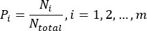(5)

where N_i denotes the number of neighboring points located in sector θ, and N_total denotes the total number of neighboring points within the spherical neighborhood. In the implementation, m = 8, corresponding to eight equal azimuthal sectors covering 0 to 2π.

To identify a sparse connected region, the cumulative point-distribution ratio of every group of λ consecutive angular sectors is calculated using circular indexing as Equation (6).

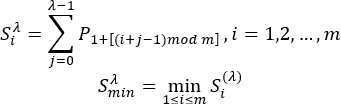(6)

Here,  denotes the cumulative point-distribution ratio of λ consecutive sectors starting from sector i. The parameter λ defines the number of consecutive sectors included in the local sparse-region search, with 1 ≤ λ ≤ m. Circular indexing is implemented using the modulo operation, so that an index exceeding the final sector wraps around to the first sector. Since m = 8 in the implementation, all sector groups are evaluated consistently within the eight-sector partition.

The modulo operation ensures that connected sectors crossing the boundary are handled continuously. If a sector is regarded as an empty region, and the current point is identified as a boundary point. If no empty sector exists, the group of consecutive sectors corresponding to is defined as the minimal connected region. Geometrically, this region represents the direction with the lowest local point density, which is more likely to correspond to the open side of a boundary. The central direction of this region is then calculated and used to guide the search toward the next candidate contour point.

Let t_min and t_max denote the indices of the first and last boundary sectors of the selected sparse region, respectively, where t_min, t_max ∈{1,…,m}. The central direction of the selected region is calculated as Equation (7).

(7)

Where  is the initial angle, and t_max and t_min represent the ending and starting positions, respectively. 2π/m is the angular width of each sector. Thus, the term 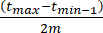 represents the angular span between the two boundary sectors, and division by two gives the corresponding central direction. When the selected region crosses the 0/2π boundary, the sector-index difference is evaluated using circular indexing, so that the index after m returns to 1.

The RANSAC (RANdom Sampling Consensus) algorithm is used for coarse registration. Any three pairs of points in the initial matching point set are selected, and the distance between the matching point pairs is represented by the inner product. For any two pairs that satisfy Equation (8), the point pairs that satisfy the distance constraint are considered to be interior points. The transformation matrix of the three pairs of points is calculated.

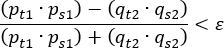(8)

In Equation (8),  and  denote source points from the two point sets, while  and  denote their corresponding target points after transformation. The subscripts s and t therefore represent the source and target, respectively, and the numerical subscripts distinguish the two corresponding point pairs. The parameter ε denotes the prescribed registration-error threshold. A correspondence is regarded as acceptable when the normalized difference between the corresponding conformal inner products is smaller than ε.

The optimal matching solution satisfies the error E and the maximum number of iterations n in Equation (9).

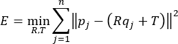(9)

Where p_j denotes the j-th target point, denotes its corresponding source point, is the rotation matrix, R is the translation vector, and T is the number of corresponding point pairs used in the registration objective. The maximum number of optimization iterations is denoted separately by N_iter. The term  represents the squared Euclidean registration error between the target point and the transformed source point.

Feature extraction layers

In SFENet, the sampling layer receives input point cloud data of size N × 3. A grouping layer follows the sampling layer, performing local neighborhood sampling based on the selected center points. The grouping layer first receives the  sampled points from the sampling layer. For each center point, the K neighboring points are aggregated to produce local point features of size , which are then passed to the feature extraction layer. The feature extraction layer consists of an MLP and a max pooling operation. The network structure of this layer is illustrated in Figure 2.

First, the point cloud data of size  from the SA layer is mapped to a 64-dimensional space using MLP in SFENet. This is followed by another MLP that further maps the features to a 1,024-dimensional space. Finally, a max pooling operation is applied to retain the maximum value along each of the 1,024 feature channels, producing a global feature representation of the point cloud. The pooling function can be expressed as in Equation (10).

  (10)

Where h(⋅) denotes the feature transformation applied to each input, g(⋅) denotes the aggregation function, and γ(⋅) denotes the subsequent learnable mapping that transforms the aggregated representation into the final feature space. Thus, γ represents a function rather than a scalar multiplication coefficient.

In SFENet, MLP is responsible for extracting point-wise features, which are then aggregated through a max pooling operation to obtain a global representation of the point cloud. To address the challenge of unordered point cloud data, the maximum value from the 1024-dimensional feature channels is selected. This ensures that the resulting feature representation is invariant to the input order of points, effectively resolving the unordered nature of point cloud inputs. By employing this approach, SFENet can more robustly process point cloud data and improve performance across various applications.

Feature processing layers

After the feature extraction layer extracts the global features from the input point cloud data, the resulting feature data has 1,024 dimensions. To facilitate subsequent classification of the processed point cloud model, the dimensionality of the feature data needs to be reduced. Based on this requirement, the feature processing layer will use the fully connected layer network structure, receiving the global feature data output by the feature extraction layer and performing dimensionality reduction on it. The feature processing network in this paper adopts a four-layer network structure, as shown in Figure 3.

As shown in the figure, the global feature data output from the feature extraction layer passes through three layers of dimensionality-reduction networks and one layer of classification evaluation network. The dimensionality-reduction network reduces the dimensionality of the global features in the point cloud data, producing low-dimensional features to support subsequent dataset construction. The classification evaluation network maps the feature data that meets the dimensionality requirements to a k-dimensional space, where each dimension represents a score for the classification accuracy of a category. The classification objective serves as a supervisory signal for feature learning and network optimization. Although the classification loss does not directly optimize contour reconstruction, it encourages the network to learn discriminative contour-aware representations that indirectly improve contour consistency and reconstruction quality.

The first layer of the feature processing layer receives 1,024-dimensional feature data from the feature extraction layer. After the first dimensionality reduction, it outputs 512-dimensional feature data. The second layer receives the 512-dimensional feature data from the first layer in the same way and reduces it to 256 dimensions. The third layer also receives the 256-dimensional data from the previous layer's dimensionality reduction and outputs 17-dimensional features. The final layer maps the resulting 17-dimensional feature data into a k-dimensional space, where k denotes the number of object categories in the classification task, and each dimension in the k-dimensional space represents the degree of match between the extracted feature data and a given object category. The intermediate feature vector is defined as ¹⁷, representing the 17 extracted feature dimensions used as the MLP input.

The loss function is used to optimize the feature learning process and guide network parameter updates. Since SFENet performs multi-category classification of point cloud targets based on extracted contour and geometric features, the output layer predicts a probability distribution over object categories. Therefore, cross-entropy loss was selected because it effectively measures the discrepancy between predicted category probabilities and ground-truth labels. This formulation is well-suited to the hierarchical feature learning pipeline in SFENet, where local and global point cloud representations are progressively fused and mapped into discriminative feature spaces. Furthermore, cross-entropy loss provides stable optimization behavior and efficient gradient propagation during training, enabling the network to learn more representative feature embeddings from contour-guided point cloud data. Its expression is expressed in Equation (11).

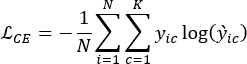(11)

Where N is the number of training samples in the corresponding batch, K is the number of object categories,  is the ground-truth indicator for sample i belonging to class c, and  is the predicted probability for class c. The cross-entropy loss is averaged over the samples within each batch.

The classification objective serves as the supervisory signal for feature learning and network optimization. The cross-entropy loss is employed to optimize the discriminative capability of the extracted point cloud features for object classification. It should be noted that this loss does not directly optimize contour reconstruction accuracy or geometric consistency. Instead, the GCE-based contour extraction module provides geometrically meaningful contour points as the input to the feature learning network, while the quality of contour extraction and reconstruction is evaluated separately through the registration and reconstruction experiments presented in the Results section. Therefore, the improvement in contour reconstruction originates from the geometry-preserving contour extraction provided by the GCE module rather than from direct optimization using a contour-specific loss function. It should be noted that the MLP is not directly trained to reconstruct contours. The cross-entropy loss supervises discriminative feature learning and classification, whereas the geometric contour localization is provided by the preceding contour extraction procedure. Contour reconstruction and registration are subsequently performed as independent downstream evaluations.

Resultaten

Datasets, setup, and metrics
This paper uses the SpaceSense-Bench³⁴ dataset as the training and testing data source for space debris point cloud feature extraction and classification algorithms. SpaceSense-Bench is a high-fidelity simulation dataset containing LiDAR point cloud data from 136 different spacecraft models, with each frame providing both a depth map and an RGB image. The dataset includes not only spatial coordinates of the point clouds but also semantic labels and precise six-degree-of-freedom (6-DoF) attitude information. The dataset contains 90,846 sparsely sampled multimodal frames. The official benchmark uses an object-level split of 117 satellite models for training, 5 for validation, and 14 for testing, ensuring that no satellite model appears in more than one subset. The validation set is used for hyperparameter tuning and early stopping, whereas the testing set is used exclusively for performance evaluation.

SpaceSense-Bench provides dense seven-class part-level semantic annotations at both the pixel and point levels. During dataset construction, spacecraft 3D meshes are decomposed into functional components and assigned semantic labels through the Stencil ID mechanism. In this study, these seven part-level semantic labels are directly adopted as the classification categories, giving k = 7: main body, solar panel, dish antenna, omni antenna, payload, thruster, and adapter ring. Therefore, the classification task predicts the semantic category of an extracted point or feature rather than the identity or global category of the complete spacecraft.

The SFENet architecture consists of three stages: Set Abstraction (SA), feature extraction, and feature processing. The SA module progressively reduces the number of sampled center points while increasing the spatial extent of local neighborhoods. The three SA stages use (N₁, r₁, K₁) = (1024, 0.10 m, 32), (N₂, r₂, K₂) = (512, 0.20 m, 64), (N₃, r₃, K₃) =  (256, 0.40 m, 128) respectively. These settings progressively aggregate local geometric information at increasingly larger spatial scales. The SA layer first samples N = 2,560 input points and groups local neighborhoods using a ball-query strategy with neighborhood sizes of 32, 64, and 128. For each sampled center point, local geometric features are aggregated and forwarded to the feature extraction stage. The feature extraction module employs shared MLP layers with dimensions of 64, 128, 256, and 1,024, with each MLP layer followed by Batch Normalization and ReLU activation. A max-pooling operation is then applied across the point features to generate a 1024-dimensional global feature vector. Subsequently, the feature-processing module uses fully connected layers with dimensions 1,024→512→256→17→k, where the 17-dimensional vector is the intermediate bottleneck representation and k = 7 denotes the number of part-level semantic categories. Thus, the MLP transforms the extracted geometric features into a compact 17-dimensional representation before producing the final seven-class semantic prediction.

To improve generalization ability and prevent overfitting, Batch Normalization was employed after each MLP layer, and dropout with a probability of 0.5 was applied to the fully connected layers during training. These regularization strategies improve training stability and reduce model sensitivity to noise.

During training, the batch size was set to 8, and the initial learning rate was initialized as 0.001 using the Adam optimizer. The learning rate was reduced using a step decay strategy during training. ReLU activation was adopted throughout the network. The model was trained for 200 epochs, and early stopping was used to avoid overfitting. All software, computational tools, datasets, hardware, and implementation resources used in the study are shown in the Table of Materials.

The reported runtime is therefore expressed as seconds per object (s/object). The runtime comparison was conducted using the same implementation environment and hardware configuration for all evaluated methods. The methods were applied to the same point-cloud inputs under identical processing conditions, and the runtime was measured for the corresponding feature extraction and contour processing procedures. No additional preprocessing or hardware acceleration was introduced selectively for SFENet. The reported runtime, therefore, reflects the processing efficiency of each method under the same experimental conditions.

Accordingly, the evaluation follows a two-level pipeline: (1) primary evaluation of feature learning and object classification, and (2) downstream evaluation of contour reconstruction and multi-view registration. The latter evaluations do not constitute direct training objectives of the MLP and are instead used to assess the geometric effectiveness of the extracted representations.

The MLP component is trained as a multi-class feature classification network using the cross-entropy loss defined in Equation (11). The classification loss supervises the learning of discriminative feature representations and does not directly optimize contour reconstruction or point cloud registration. Therefore, contour reconstruction and registration are treated as downstream geometric evaluation procedures. After feature learning, the extracted contour candidates are reconstructed and registered across multiple views, and the resulting geometric errors are used to evaluate the quality of the extracted contour information. This separation between the learning objective and geometric evaluation is important for interpreting the experimental results.

The Root Mean Square Error (RMSE) is used to evaluate the registration accuracy between two aligned point clouds, as shown in Equation (12).

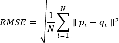  (12)

Where N denotes the number of corresponding point pairs after registration, p_i is the i-th point in the registered point cloud, and q_i is the corresponding ground-truth point. A lower RMSE indicates more accurate point cloud registration. The correspondences are generated by the multi-view registration procedure. The resulting RMSE is reported in centimeters (cm).

Contour reconstruction error measures the geometric distance between the reconstructed and their corresponding reference contour points. For contour correspondences, it is calculated as Equation (13).

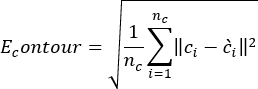(13)

Where and denote the reference and reconstructed contour points, respectively. Correspondences are established between reconstructed and reference contour points according to the nearest-point correspondence rule. This error is reported in centimeters (cm).

Contour length error measures the relative difference between the reconstructed contour length and the reference contour length, as shown in Equation (14).

  (14)

Where and denote the reconstructed and reference contour lengths, respectively. This metric is reported as a percentage (%) and does not require point-to-point correspondence.

Overall Accuracy (oAcc) and Mean Class Accuracy (mAcc) are adopted to evaluate the classification performance of SFENet. Assume that the test dataset contains C object categories. Let TP_i denote the number of correctly classified samples belonging to category i, and FN_i denote the number of samples belonging to category but incorrectly classified into other categories. The total number of test samples is given by .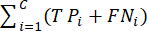

The Overall Accuracy (oAcc) measures the proportion of correctly classified samples among all test samples and is defined as Equation (15).

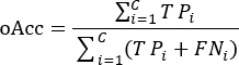  (15)

The Mean Class Accuracy (mAcc) evaluates the average classification accuracy over all categories and is defined as Equation (16).

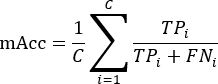  (16)

Where C is the total number of object categories, TP_i is the number of correctly classified samples in category i, and FN_i is the number of samples belonging to category i that are misclassified into other categories. A higher oAcc indicates better overall classification performance, while a higher mAcc reflects more balanced classification performance across different categories, making it less sensitive to class imbalance.

The rotation experiment uses 16 frames from one spacecraft model, corresponding to the predefined viewpoint rotation conditions. Three repeated trials were conducted for each rotation condition. The ground-truth rotation error was calculated by comparing the estimated rotation matrix R_est with the ground-truth rotation matrix R_gt as Equation (17).

  (17)

And the rotation error is obtained from its corresponding rotation angle as Equation (18).

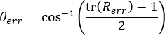(18)

The resulting rotation error is reported in degrees (°).

Since contour reconstruction is not directly optimized during training, the effectiveness of the proposed geometry-guided framework is evaluated indirectly through multi-view registration accuracy (RMSE), contour reconstruction quality, and feature classification performance (oAcc and mAcc). These complementary evaluations demonstrate the quality of the extracted contour representations from both geometric and recognition perspectives. It should be noted that contour reconstruction is not included as a direct optimization objective during network training. The network is trained using multiclass cross-entropy loss, whereas contour reconstruction and registration are performed post-hoc to evaluate the geometric quality of the extracted contour candidates. Therefore, the RMSE and registration results should be interpreted as downstream evaluations of the proposed feature extraction framework rather than as losses directly minimized during training.

Ablation experiments

To investigate the contribution of each component in SFENet, ablation experiments were conducted to separately analyze the effects of GCE-based geometric processing, MLP-based feature learning, and contour-guided strategies. In the Baseline, only the MLP is used without GCE or contour guidance. In GCE + MLP, the geometrically extracted contour information is provided to the MLP, but the contour-guided strategy is not additionally applied. In MLP + contour-guided, contour guidance is applied to the MLP without activating the GCE module. Finally, SFENet combines GCE, MLP feature learning, and the contour-guided strategy. The experimental results are summarized in Table 1. All ablation and comparison experiments were conducted using the same training, validation, and testing splits, network architecture, optimizer, and hyperparameter settings. To clarify the ablation settings, the three components in Table 1 represent different stages of the proposed framework. GCE performs geometry-guided contour extraction from the input point cloud. MLP performs feature learning and classification using the resulting feature representation. The contour-guided strategy uses contour-related information to guide the feature-learning process. It does not introduce an additional mask, auxiliary loss, or feature-weighting operation, and all configurations use the same cross-entropy classification objective. Therefore, the ablation study evaluates the individual and combined effects of geometric contour extraction and contour-guided feature learning.

As shown in Table 1, incorporating the GCE module significantly improves contour extraction accuracy and overall performance. By preserving geometric structures and reducing the inclusion of non-contour points, GCE-based contour preprocessing yields more reliable localization of contour candidates, thereby reducing registration mismatches and improving contour consistency. The MLP module contributes by learning discriminative local and global feature representations, enhancing the robustness of the framework under varying target poses and complex environments. The contour-guided strategy further improves contour continuity and reconstruction quality by constraining feature learning using contour information. The complete SFENet framework obtains the best results across all evaluation metrics. These findings demonstrate that the performance gains arise from the complementary interaction of geometry-guided contour extraction, feature learning, and contour-driven processing.

Multi-view registration was performed using a coarse-to-fine strategy consisting of RANSAC-based initial alignment followed by ICP refinement³⁵. Point cloud frames were generated from different observation viewpoints around the target, and contour point clouds extracted from adjacent views were subsequently registered. Registration accuracy was evaluated using RMSE between corresponding contour points after alignment.

To evaluate the effect of the number of views on multi-view registration, five registration levels are considered. Level 1 involves registration between two adjacent views and represents the basic pairwise registration case. Level 2 uses three consecutive views to evaluate registration consistency across multiple views. Level 3 involves four consecutive views and provides a more challenging multi-view registration configuration. Level 4 uses five consecutive views to further evaluate the accumulation of registration errors. Level 5 includes all available views and represents the complete multi-view registration scenario used for final contour reconstruction. This progressive design enables evaluation of registration performance as the number of views and geometric complexity increase. Table 2 shows the RMSE of the contour point cloud, the original point cloud, and the multi-view registration using the Fast Point Feature Histogram (FPFH) + ICP method³⁶.

The contour-based method used in SFENet yields significantly lower registration errors compared with original point cloud registration and FPFH-based registration approaches. This is because the ICP registration method, used for overall model reconstruction, requires a high degree of overlap. Contour reconstruction, on the other hand, fully leverages contour features, thereby reducing the mismatch rate and improving matching speed and accuracy. FPFH relies on the accuracy of normal calculation, requires the establishment of a local coordinate system, and demands a relatively uniform point cloud distribution. The high curvature similarity in many areas leads to a significant reduction in the expressiveness and discriminative power of the descriptors.

Initial sampling points are the points initially selected for input to the SFENet network. Since some data of point clouds are often dense, containing a large number of points, using all points as network input is not only computationally intensive but may also be difficult for the network to process. Therefore, in practical applications, a sampling strategy is typically used as initial sampling points, which are then used as network input. This reduces computation while ensuring the network learns features. However, overly sparse sampling points cannot represent the global features. Given the computational limitations of the experimental conditions in this paper, four sample sizes were selected for simulation. The results are shown in Table 3.

As the number of sampled points increases, overall performance generally improves, although slight fluctuations are observed. Specifically, the oAcc decreases slightly from 0.918 to 0.915, then increases to 0.920 and 0.930 at higher sampling densities. This result suggests that increasing the number of sampled points generally benefits feature extraction and classification performance, but the improvement is not strictly monotonic. Furthermore, when N = 2,560, both oAcc and mAcc reach their maximum values simultaneously. This indicates that in the application environment described in this paper, the more initial sampling points there are, the stronger the feature extraction model's recognition and classification ability, and the more accurate the shape feature data extracted for the target. In the simulation comparison experiment described below, the initial number of sampling points was set to 2,560.

The number of ball query points is significant for training the feature network, directly determining the size of local regions during point cloud feature fusion. If the number of ball query points is too large, the fused local features of the point cloud data will be too large, which is not conducive to extracting detailed features. Similarly, in many cases, even when points far apart are classified into the same category, the features they describe may not be similar. Furthermore, the number of ball query points is proportional to the overall computational cost. Considering the influence of various factors, this paper sets four sets of ball query point numbers for the SA layer and conducts related classification experiments. Since the ball query algorithm in this paper involves three layers of ball query methods, each targeting different ball radii, the number of ball query points involves three layers of parameters. The results for various ball query points are shown in Table 4.

Experimental results show that the oAcc and mAcc values do not simply increase with the number of query points. Instead, they reach their maximum values under a specific combination of query-point counts. Subsequently, as the number of query points increases, both oAcc and mAcc decrease. The oAcc and mAcc values reach their maximum when the number of query points is (32, 64, 128), at which point the feature extraction model exhibits the strongest recognition and classification ability. As the ball-query neighborhood size increases, the performance does not improve monotonically. The decline observed at larger neighborhood sizes may indicate that excessively large neighborhoods reduce the discriminative nature of local geometric features by incorporating less relevant points. However, since Table 4 does not include training–validation curves, this observation should not be interpreted as direct evidence of overfitting.

Comparison experiments

To comprehensively evaluate the effectiveness of SFENet, comparisons were conducted using both traditional contour extraction approaches and representative deep learning-based point cloud methods. The selected approaches include KNN¹², 3D-gradient³⁷, image-based contour extraction³⁸, PointNet³⁹, PointNet++⁴⁰, PointNeXt¹⁹, and our proposed SFENet. Traditional methods mainly rely on local geometric properties or projection-based processing, whereas deep learning approaches learn feature representations directly from point cloud data.

Among the compared methods, PointNet employs shared multilayer perceptrons and global pooling operations for point-wise feature extraction. PointNet++ further introduces hierarchical neighborhood grouping and multi-scale feature learning to improve local structure representation. PointNeXt enhances PointNet-family architecture through optimized training strategies and improved feature aggregation mechanisms. In contrast, KNN, 3D-gradient, and image-based methods explicitly utilize geometric information for contour extraction but have limited feature-representation capability. SFENet integrates GCE-based contour candidate extraction with MLP-based hierarchical feature learning, combining geometric priors with learned representations. The quantitative comparison results are shown in Table 5. Since the compared methods have different intrinsic outputs, a unified downstream evaluation procedure is used to obtain comparable metrics. PointNet, PointNet++, and PointNeXt are learning-based point cloud networks that provide feature representations and classification predictions but do not inherently perform contour reconstruction. For these methods, the same downstream contour-generation procedure is applied to obtain the contour required for RMSE evaluation. KNN, 3D-gradient, and image-based contour methods are non-learning-based contour-extraction approaches and therefore do not include an intrinsic object-classification head. For these methods, the same downstream classifier is applied to the extracted contour-related features to obtain oAcc and mAcc. The same data preprocessing, evaluation samples, and metric definitions are used across methods wherever applicable. All methods were evaluated using the same input data, preprocessing procedure, and metric definitions. Learning-based methods were trained on the specified training set, whereas non-learning-based methods were evaluated directly without a training stage. Common downstream classification or contour-generation procedures were used where necessary to obtain comparable metrics.

The traditional contour extraction methods generally exhibit lower classification performance and larger contour reconstruction errors. Although KNN achieves relatively higher accuracy among traditional methods, it requires neighborhood traversal operations, which increase computational cost. The 3D-gradient method relies heavily on local curvature variations and is sensitive to contour noise, whereas the image-based method suffers from information loss due to projection from three-dimensional space to two-dimensional representations. Compared with conventional approaches, deep learning methods significantly improve feature representation capability. PointNet achieves improved classification accuracy through point-wise feature learning, while PointNet++ and PointNeXt further enhance performance by capturing hierarchical and multi-scale geometric information. PointNeXt achieves stronger performance than PointNet and PointNet++ due to its optimized feature aggregation strategy.

SFENet achieves the best overall performance across all evaluation metrics, obtaining an oAcc of 0.930, mAcc of 0.869, and the lowest RMSE of 0.173 cm. SFENet achieves a slightly higher oAcc than PointNeXt (0.930 vs. 0.925) under the reported experimental setting. Because the results are obtained from a single split/run, this difference should be interpreted as an observed performance difference rather than a statistically significant improvement. Moreover, SFENet has a runtime of only 1.65 s, which is lower than that of most learning-based approaches. The superior performance of SFENet can be attributed to the complementary interaction between GCE-based geometric contour extraction and MLP-based feature learning.

Although the above results demonstrate the overall superiority of SFENet against both traditional and learning-based methods, the primary objective of this work is to learn discriminative feature representations from geometry-guided contour information and perform object classification. Contour reconstruction and multi-view registration are used as downstream geometric evaluations to assess the usefulness of the learned features. Therefore, a more detailed analysis was further conducted using four representative contour extraction approaches: KNN, 3D-gradient, image-based methods, and SFENet. These methods directly operate on contour localization and geometric reconstruction, allowing a more comprehensive evaluation of robustness, contour extraction quality, and geometric accuracy under different target poses and environmental conditions. The following experiments analyze the performance of these four methods from three perspectives: registration robustness under varying viewing angles, contour reconstruction quality, and contour extraction accuracy. The parameter settings for each method are shown in Table 6, including K of KNN, Nearest Point Set (M), and Neighborhood radius (R) of 3D gradient-based point cloud feature extraction, and Region Growth (θ), Regional merging (γ), and θ of the image-based contour extraction method.

The following procedure was followed to evaluate the robustness. First, the outer contours of 16 point cloud frames were extracted using SFENet and the other three methods. Then, the point cloud contours, rotated in different poses (rotation angles about the y-axis ranging from -75° to 75° in 15° increments), were registered to the original point cloud model. Finally, the registration accuracy of each method across different poses was evaluated for rotation about the y-axis. The results are shown in Figure 4. The robustness evaluation in this work focuses on viewpoint variations, rotating the target about the Y-axis while keeping the remaining sensing conditions unchanged. This experiment is intended to evaluate the stability of the proposed contour extraction and feature learning framework under different observation angles. Other practical sensing factors, including measurement noise, outlier points, missing observations, non-uniform point density, sparse sampling, partial occlusion, varying point counts, and different sensor-view distances, are beyond the scope of the current study and are left for future investigation.

As shown in Figure 4, the rotation angle errors of each method differ significantly under different Y-axis rotation angles. Overall, SFENet maintains near-zero error across the entire angle range, with a maximum rotation-angle error of 0.073°, demonstrating the strongest stability and robustness. The KNN method has relatively small errors, but fluctuates slightly with increasing rotation angle, making its stability less than that of SFENet. Methods based on initial point clouds and images show significant increases in error over medium to large angle ranges, especially above ±40°, indicating their sensitivity to rotational changes. In contrast, the 3D-gradient method exhibits large error peaks at certain angles, showing greater overall fluctuation and poorer robustness. In summary, SFENet achieves improved performance in contour extraction and classification under the evaluated simulation and viewpoint-rotation conditions. Its robustness to noise, missing observations, outliers, occlusion, point-density variation, and sensor characteristics remains to be further validated. The key reason for this lies in its contour point extraction method based on GCE, which preserves the geometric features of the original outer contour to the greatest degree, thereby effectively reducing the mismatch rate and improving contour registration accuracy.

This work also compares the contour length extracted by SFENet with that of the reference model and uses the error as the evaluation criterion. In the experiment, the satellite model was divided into 20 local contour segments. The examples of final contour point extraction are shown in Figure 5. The comparison of relative scale errors on contour points is shown in Figure 6, which shows the relative errors of SFENet and the other three algorithms in each contour segment. The results show that the contour extracted by SFENet is closer to the reference model at each scale.

Specifically, the edges obtained by the 3D-gradient method are relatively wide, similar to the thick and bright edges produced by the Sobel operator in image processing. The Based-image method projects the 3D point cloud onto a 2D plane and then applies an image edge-extraction algorithm, thereby altering the contour model structure. This is mainly because the "scale" parameter in this method is not sufficiently adaptable to irregular point cloud densities, leading to deviations in the positions of contour points. The contour points obtained by the KNN method are too sparse and include few non-contour points.

SFENet's superior performance is primarily due to two factors. First, the starting point for the boundary sphere search is selected from geometric feature points, which are typically located on the model's outer contour. When parameters are set appropriately, the search direction largely follows the contour line, minimizing deviation. In contrast, methods that do not fully utilize point cloud geometric features are prone to introducing non-contour points. Second, GCE characterizes spatial relationships among neighboring points by evaluating occupancy in eight azimuthal sectors of a local spherical neighborhood, enriching the feature description of contour points. While based-image methods also utilize point normals and curvature for feature description, they only reflect the overall features of the point and its neighborhood, failing to fully express the spatial structure of the contour.

Although a detailed robustness analysis focuses on four primary contour extraction methods (KNN, 3D-gradient, image-based, and SFENet), additional classical approaches are included to provide a broader performance reference and context. Table 7 compares the performance of representative contour extraction methods under different geometric processing strategies from running time (t), number of contour points (N), minimum error (Emin), maximum error (Emax), average error (Eaver), average relative error (Raver), and RMSE. Results show that SFENet significantly outperforms other methods in overall RMSE.

It should be noted that the Based-image method calls image-processing functions in the Point Cloud Library (PCL), which is slightly faster than SFENet in terms of computation time, but it produces a fitted contour rather than the original contour points, leading to deviations in contour position. The contour points from the 3D gradient are coarser, and after straight-line fitting, they also deviate from the original point cloud positions. Although the KNN method has relatively small errors, it requires traversing all points, resulting in longer computation time. In contrast, SFENet retains only candidate contour points in each search, keeping their spatial locations and geometric features unchanged. The search direction expands along the boundary, eliminating the need to traverse all points, thus achieving higher speed and accuracy.

The above experiments systematically compared SFENet with other methods in terms of algorithm robustness, contour extraction results, and contour scale error. SFENet's method of searching candidate contour points using boundary spheres uses eight-sector azimuthal searching along the boundary to preserve the spatial positional relationships and geometric structural features of contour points, providing favorable conditions for the reconstruction of 3D contour models. Moreover, the most time-consuming step in contour extraction is the search for contour points, and SFENet does not evaluate each point in the point cloud individually. Its search direction, according to the algorithm's design, always expands along the boundary region and proceeds through the eight azimuthal sectors rather than six, thus reducing computational time. By leveraging positional relationships among point cloud polyhedra to identify concave and convex points, SFENet can extract the external strip contour of the point cloud model at a scale closer to the reference model. In summary, SFENet not only preserves the geometric features of the original model in contour extraction but also significantly reduces interference from non-contour points, improving the accuracy and robustness of contour reconstruction.

Although SFENet demonstrates promising performance on the SpaceSense-Bench dataset, the current validation is limited to a high-fidelity simulation environment. The experiments do not include real, measured space debris point clouds or practical sensing conditions, such as incomplete observations, non-uniform point-cloud density, varying sensor characteristics, or different levels of measurement noise. Therefore, the reported results should be regarded as a verification of the feasibility and effectiveness of the proposed framework under simulation conditions rather than as evidence of its performance in real operational scenarios.

Data Availability:

All experimental results reported in this study were based on the SpaceSense-Bench dataset. SpaceSense-Bench is publicly available at https://github.com/wuaodi/SpaceSense-Bench. The source code, including scripts, configuration files, and dataset splits, is available at https://github.com/YaoDalei-pro/SFENet_main/tree/main/SFENet.

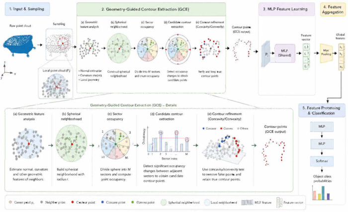
Figure 1. The overall structure of SFENet. The framework consists of five stages (1) input and sampling; (2) geometry-guided contour extraction; (3) MLP-based feature learning; (4) feature aggregation; (5) feature processing and classification. Abbreviations: GCE = geometry-guided contour extraction; MLP = multilayer perceptron; SFENet = Space Debris Point Cloud Feature Extraction Network. Please click here to view a larger version of this figure.

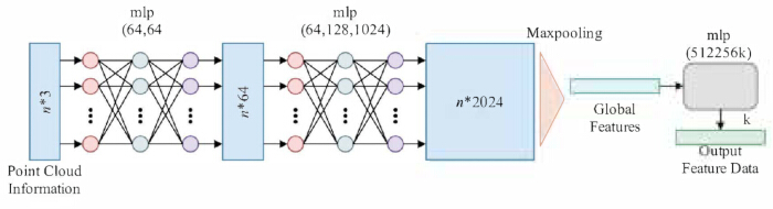
Figure 2. The network structure of MLP-based feature extraction layers. Abbreviation: MLP = multilayer perceptron. Please click here to view a larger version of this figure.

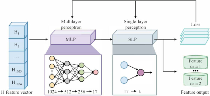
Figure 3. The network of MLP-based feature processing layers. Abbreviation: MLP = multilayer perceptron. Please click here to view a larger version of this figure.

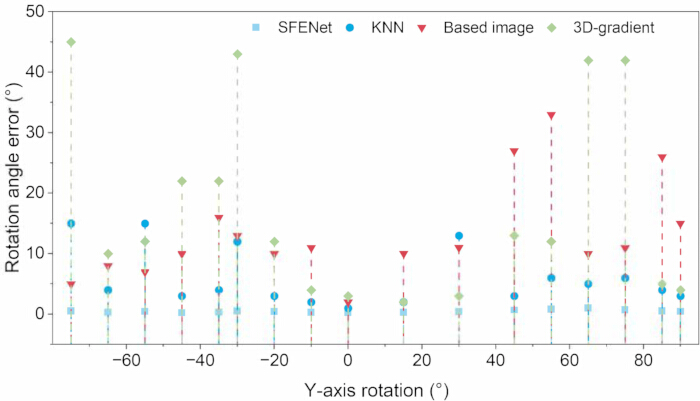
Figure 4. Robustness test of contour point cloud registration. Please click here to view a larger version of this figure.

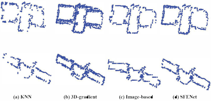
Figure 5. Examples of final contour point extraction of four methods. Please click here to view a larger version of this figure.

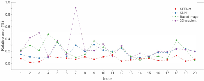
Figure 6. Comparison of relative scale errors of four methods. Please click here to view a larger version of this figure.

Configuration	GCE	MLP	Contour-guided strategy	RMSE (cm) ↓	oAcc ↑	mAcc ↑
Baseline	×	✓	×	0.244	0.903	0.824
GCE + MLP	✓	✓	×	0.216	0.919	0.845
MLP + contour-guided	×	✓	✓	0.227	0.912	0.84
SFENet	✓	✓	✓	0.173	0.93	0.869

Table 1: Ablation study of individual module contributions in SFENet. Abbreviation: SFENet = Space Debris Point Cloud Feature Extraction Network. Abbreviations: GCE = geometry-guided contour extraction; MLP = multilayer perceptron; oAcc = overall accuracy; mAcc = mean accuracy.

Level	1	2	3	4	5
Feature
Viewpoint overlap (%)	20	40	60	80	100
Outline	0.0126	0.009	0.0087	0.005	0.0036
Original point cloud	0.0169	0.0119	0.0118	0.006	0.0047
FPFH	0.0238	0.0187	0.0153	0.0083	0.0059

Table 2: RMSE (m) comparison of different contour representations in multi-view registration. Abbreviations: RMSE = root mean square error; FPFH = Fast Point Feature Histogram; ICP = Iterative Closest Point.

Indicators	N=1024	N=1536	N=2048	N=2560
oAcc	0.918	0.915	0.92	0.93
mAcc	0.823	0.825	0.83	0.869

Table 3: Experimental results at different sampling points.

Indicators	(16, 32, 64)	(32, 64, 128)	(64, 64, 128)	(64, 128, 128)
oAcc	0.927	0.93	0.917	0.92
mAcc	0.857	0.869	0.829	0.841

Table 4: Experimental results under different numbers of ball query points.

Method	oAcc ↑	mAcc ↑	RMSE (cm) ↓	Runtime (s)
KNN	0.864	0.782	0.409	11.19
3D-gradient method	0.839	0.748	0.459	2.67
Image-based method	0.811	0.691	0.6	1.46
PointNet	0.904	0.835	0.267	2.33
PointNet++	0.918	0.844	0.236	2.84
PointNeXt	0.925	0.852	0.209	3.15
SFENet	0.93	0.869	0.173	1.65

Table 5: Performance comparison with traditional and deep learning-based point cloud methods. Abbreviations: KNN = k-nearest neighbors; FPFH = Fast Point Feature Histogram; GCE = geometry-guided contour extraction; MLP = multilayer perceptron; oAcc = overall accuracy; mAcc = mean accuracy; RMSE = root mean square error.

KNN	3D-gradient method		Image-based method
K	M	R	θ	γ	tho
30	30	20d	35°	45°	3 scale

Table 6: The parameter settings of the compared methods. Abbreviation: KNN = k-nearest neighbors.

Algorithm	t (s)	N	Emin (cm)	Emax (cm)	Eaver (cm)	Raver	RMSE (cm)
KNN	11.19	234	0.871	2.804	0.863	0.064	0.409
3D-gradient method	2.67	845	0.385	4.766	0.888	0.171	0.459
Image-based method	1.46	522	0.55	8.013	1.314	0.107	0.6
SFENet	1.65	449	0.069	1.694	0.089	0.052	0.173

Table 7: Comparison of four methods in contour extraction. Abbreviations: KNN = k-nearest neighbors; RMSE = root mean square error; SFENet = Space Debris Point Cloud Feature Extraction Network.

Discussie

The quantitative evaluation was conducted exclusively on the SpaceSense-Bench simulation dataset. Therefore, the results demonstrate performance under controlled simulation conditions rather than robustness to real LiDAR measurements. Real sensor data may involve noise, non-uniform sampling, missing points, occlusion, and sensor- or surface-dependent variations, which could affect both geometry-guided contour extraction and MLP-based feature learning. Although the proposed framework operates on local spatial relationships and point distributions and is therefore potentially transferable to real point clouds, such transferability remains to be experimentally verified.

An important distinction is that SFENet is trained using multiclass cross-entropy loss for feature learning and classification. Contour reconstruction and multiview registration are not included in the training objective but are performed post-hoc to evaluate the geometric quality of the extracted features. Thus, the reported contour reconstruction accuracy should not be interpreted as direct optimization of contour reconstruction, but as evidence that the extracted geometric information provides useful input for subsequent reconstruction and registration.

The current experiments also do not evaluate robustness to noise, missing observations, outliers, occlusion, non-uniform point density, or different sensor configurations. Future work will therefore validate SFENet using real or publicly available LiDAR point clouds and cross-dataset testing from simulated to real measurements. Additional experiments will vary point density, noise, missing data, and sensor configurations, with evaluation based on classification performance, contour reconstruction error, and registration accuracy. These experiments will determine whether the performance observed on SpaceSense-Bench can be maintained under realistic sensing conditions.

In conclusion, this paper proposes the SFENet model for feature extraction and contour reconstruction of space debris point clouds based on geometry-guided contour extraction and a Multilayer Perceptron. SFENet improves candidate contour point extraction by introducing GCE to unify the geometric relationships of point clouds. Simultaneously, it utilizes MLP to efficiently fuse local and global features. Experimental results show that SFENet achieves an RMSE of 0.173 cm in contour extraction under simulation conditions, demonstrating its effectiveness for space debris contour reconstruction and feature representation. Overall, SFENet provides a geometry-guided approach for contour extraction and feature representation of space-debris point clouds, with potential relevance to subsequent perception and geometric reconstruction tasks. However, the current evaluation is limited to simulation data and does not establish robustness under realistic sensing conditions. Future work will evaluate the framework using real or laboratory-acquired LiDAR point clouds, with particular attention to noise, incomplete observations, non-uniform point density, occlusion, and sensor variation, to further assess its generalization and practical applicability.

Materialen

Lijst van materialen gebruikt in dit artikel

Naam	Bedrijf	Catalogusnummer	Opmerkingen
Intel Core i5-9600K CPU	Intel Corporation	i5-9600K	3.70 GHz; used with 8 GB RAM for all experiments.
NVIDIA GeForce GTX 1650 GPU	NVIDIA Corporation	GTX 1650	Used for network training and inference.
Point Cloud Library (PCL)	Open Perception Foundation	N/A	Image-based baseline, RANSAC, ICP, and FPFH. https://pointclouds.org
Python	Python Software Foundation	3.7	Runtime environment. https://www.python.org
PyTorch	PyTorch project	N/A	SFENet and learning-based baselines; Adam, BatchNorm, ReLU, dropout (p = 0.5), cross-entropy. https://pytorch.org
SpaceSense-Bench	Wu et al.	arXiv:2603.09320	Training/validation/test dataset and toolkit. https://github.com/wuaodi/SpaceSense-Bench ; https://huggingface.co/datasets/Alvin16/SpaceSense-Bench
Ubuntu 18.04 LTS	Canonical Ltd.	18.04 (64-bit)	Host operating system. https://ubuntu.com