A Step-by-Step Protocol for Quantifying Molecular Forces in Living Cells Using the Vinculin TSMod FRET Tension Sensor

Resumo

This protocol describes stepwise expression, imaging, and quantitative analysis of the vinculin TSMod FRET tension sensor to map piconewton forces in living cells. It details culture conditions, acquisition of ratiometric and spectral FRET data, image processing for accurate FRET quantification, and application to focal adhesion mechanobiology.

Resumo

Genetically encoded FRET-based tension sensors provide a powerful approach for visualizing and quantifying molecular forces within living cells. These probes incorporate an extensible, calibrated elastic linker between a donor-acceptor fluorophore pair, enabling mechanical load changes to be reported as variations in FRET efficiency. This article presents a detailed, stepwise protocol for the expression, imaging, and quantitative analysis of the vinculin tension sensor (VinTS), which reports forces transmitted through vinculin within focal adhesions. The procedure describes optimized conditions for cell culture and guidelines for selecting appropriate imaging modalities, and recommendations for acquiring high-quality ratiometric or spectral FRET datasets. In addition, the workflow includes image processing steps for background subtraction, bleed-through correction, FRET ratio calculation, and spatial mapping of tension across adhesion sites. Representative results illustrate how VinTS can be used to assess cytoskeleton-dependent mechanical forces and to correlate tension distribution with adhesion assembly and maturation. While demonstrated here for vinculin, the methodological framework is readily adaptable to other FRET-based tension sensors and mechanosensitive proteins.

Introdução

Mechanical forces are fundamental regulators of multicellular organization, acting together with biochemical signals to shape tissue development, homeostasis, and repair¹. During morphogenesis, cells continuously generate, transmit, and interpret mechanical cues through specialized molecular assemblies², a process known as mechanotransduction, which converts physical forces into biochemical signals that govern cell fate, migration, and collective behavior³. Despite its central role in biology, a major challenge remains to identify and quantitatively probe the primary mechanotransducers, i.e., the molecules that directly experience mechanical load and initiate force-dependent signaling.

Genetically encoded FRET-based molecular tension sensors provide a powerful strategy to address this challenge by enabling direct measurement of piconewton-scale forces acting on individual proteins in living cells and tissues⁴. In molecular tension microscopy (MTM), an extensible, calibrated elastic linker flanked by a donor-acceptor pair is inserted into a protein of interest⁴, such that mechanical stretching of the linker increases the distance and/or reorientation between fluorophores and decreases FRET efficiency in a force-dependent manner⁵. When combined with quantitative imaging approaches, these biosensors function as molecular strain gauges that report molecular tension with high spatial and temporal resolution⁶.

Early generations of MTM sensors employed elastomeric polypeptides derived from spectrin repeats or spider silk, e.g., the tension sensor module (TSMod), which behave as entropic springs with well-characterized force-extension relationships and are therefore amenable to calibration in the 1–10 pN range^4,7. When combined with quantitative imaging approaches such as fluorescence lifetime imaging microscopy (FLIM) or acceptor-sensitized emission, these sensors have enabled dynamic mapping of force distributions within single living cells^8,9. In particular, intensity-based spectral FRET measurements are particularly attractive in this context, because they simultaneously capture donor quenching and reciprocal acceptor excitation, thereby providing a robust ratiometric readout of force-dependent conformational changes⁶. In practice, such measurements are often performed using conventional widefield epifluorescence microscopy. This approach is intrinsically more sensitive to optical cross-talk and illumination heterogeneity, both of which can compromise the accuracy and reproducibility of FRET quantification. Careful calibration using appropriate controls, such as donor-only and acceptor-only samples, is therefore essential to correct for bleed-through and ensure reliable quantification¹⁰. By comparison, spectral confocal imaging provides narrower detection channels that improve donor–acceptor discrimination and reduce bleed-through, spectral overlap, and background autofluorescence. This is particularly advantageous for focal adhesion imaging, where the structures of interest are small, spatially restricted, and confined to a thin ventral optical plane, making strong optical sectioning especially important for reliable quantification.

The versatility of FRET-based tension sensors has led to their application to a growing number of mechanically active proteins, including core cytoskeleton components such as actin, α-actinin, spectrin, and filamin^11,12,13, as well as adhesion-associated proteins such as vinculin, E-cadherin, VE-cadherin, and PECAM-1^14,15,16,17. More recently, similar strategies have been extended to extracellular structures such as collagen and elements of the glycocalyx¹⁸. A systematic compilation of SSP-based TSMod biosensors applied across mechanosensitive proteins, fluorophore pairs, and experimental systems is provided in Supplementary Table 1; this table is restricted to sensors incorporating a spider silk protein linker and explicitly excludes tension biosensors based on alternative elastic modules, including STReTCh¹⁹, PILATeS²⁰, spectrin repeats^7,11,21, loop domains²², and (GGSGGS)_n linkers²³. Across experimental systems ranging from two-dimensional cell cultures to whole organisms such as Caenorhabditis elegans and Drosophila melanogaster, MTM has provided direct evidence that mechanical forces are dynamically regulated across multiple scales and compartments during development and tissue remodeling^24,25.

A critical requirement in MTM-based studies is that insertion of the FRET module does not perturb the native function of the host protein. Rigorous validation is therefore essential and typically includes biochemical verification of protein integrity, proper subcellular localization, and assessment of dynamic behavior using approaches such as fluorescence recovery after photobleaching (FRAP). Functional rescue experiments in loss-of-function backgrounds provide the most stringent test that the biosensor-tagged protein remains competent to support complex biological processes⁸. In parallel, force-insensitive and tensionless controls are required to distinguish genuine mechanosensitive changes in FRET from environmental or photophysical artifacts²⁶.

Among the proteins studied to date, vinculin represents a prototypical mechanotransducer that localizes to focal adhesions and adherens junctions, where it mechanically links adhesion receptors to the actin cytoskeleton. Mechanical force can promote vinculin engagement with adhesion components and strengthen coupling between the extracellular matrix or neighboring cells and the cytoskeleton. Vinculin adopts conformations that enable binding to partners such as talin, actin, and other signaling proteins, thereby supporting focal adhesion maturation, epithelial cohesion, and coordinated collective cell migration⁴. Studies from several groups have shown that vinculin tension is associated with adhesion remodeling and collective cell behaviors, supporting its role as a mechanosensitive regulator of tissue organization^27,28,29,30.

In this study, we present a three-day experimental workflow for quantifying molecular tension at vinculin using a genetically encoded FRET-based tension sensor module (VinTS). All image data generated for this manuscript are original and have not been previously published. Building on previously established TSMod-based vinculin sensors and molecular tension microscopy approaches^8,31, this protocol provides a streamlined framework for the accurate interpretation of FRET signals in the context of molecular force transmission within living cells. Although the protocol is developed for vinculin, the methodological framework is readily adaptable to other TSMod-based tension sensors and mechanosensitive proteins.

Protocolo

Experiments were performed in Madin–Darby canine kidney (MDCK) epithelial cells stably expressing wild-type or mutant variants of the vinculin tension sensor (VinTS). As schematized in Figure 1A, VinTS consists of the TSMod inserted between the vinculin head (Vh) and tail (Vt) domains. An example of the VinTS emission spectrum obtained in MDCK cells is shown in Figure 1B, with the donor and acceptor emission peaks indicated. The mutant constructs include the tail-less control VinTL, which lacks amino acids beyond residue 883 required for tail-mediated interactions³². VinTL disrupts force-bearing interactions with actin and thus does not support actin-based tensile loading, although it may still experience other mechanical forces, such as compression³³. In addition, we analyzed two previously characterized vinculin mutants that alter mechanosensitivity or force transmission: VinT12, containing four charge-to-alanine substitutions in the tail domain (D974A:K975A:R976A:R978A) that impair the head-tail interaction³⁴, and VinV1001A, bearing a valine-to-alanine substitution at residue 1001 in Vt that reduces actin binding without disrupting vinculin autoinhibition³⁵. Previous work using vinculin tension sensors has shown that related tail-domain mutants such as I997A are also effectively unloaded, consistent with strongly reduced actin binding³⁶, highlighting valine/isoleucine substitutions in this region as robust actin-binding–deficient controls.

In this protocol, the VinTL control, in which the module is expressed in a non-force-bearing configuration, establishes the maximum FRET efficiency, whereas force-insensitive or constitutively open variants such as VinV1001A and VinT12, respectively, serve to calibrate the sensor response to actin-mediated pulling forces. FRET standards are also stably expressed in MDCK cells for system calibration: 5AA (mTFP1-GPGGA-Venus) and TRAF (mTFP1-TRAF-Venus)³⁷.

Perform the experimental workflow over three consecutive days. On Day 1, perform cell culture and seeding on different substrates. On Day 2, perform live-cell spectral FRET imaging to capture dynamic vinculin tension at focal adhesions. On Day 3, perform image processing and FRET quantification, enabling relative measurement of vinculin tension across constructs.

1. Day 1: cell culture, detachment, and seeding for live-cell imaging

1. Preparation of cell culture and imaging medium
   1. Prepare Dulbecco’s Modified Eagle Medium (DMEM) supplemented with 10% fetal bovine serum (FBS), 1% penicillin/streptomycin, and 1% L-glutamine (referred to as complete growth medium).
   2. Prepare a complete imaging medium (referred to as imaging medium) by supplementing FluoroBrite DMEM with 1% L-glutamine, 1% penicillin/streptomycin, 10% FBS, and HEPES (optional) to a final volume of 50 mL, and store at 4 °C for up to 1 month.
      NOTE: FluoroBrite DMEM was used for live-cell imaging due to its low autofluorescence.
      CAUTION: Protect the imaging medium from light by using opaque tubes or aluminum foil. When imaging was performed outside a 5% CO₂-controlled environment, buffer the medium to pH 7.4 with 20 mM HEPES.
   3. Warm all media and solutions to 37 °C prior to use.
2. Cell culture maintenance
   1. Culture MDCK cells in a humidified incubator at 37 °C with 5% CO₂. If starting from frozen stocks, thaw cells at least 8 days before experiments. Monitor cells regularly and passage them when they reach 70–80% confluence.
3. Cell detachment
   1. Pre-equilibrate a new T25 flask containing 4.5 mL of fresh complete growth medium in the incubator. Aspirate the spent medium from the cell culture flask.
   2. Wash cells once with 1 mL of Ca²⁺/Mg²⁺-free phosphate-buffered saline (PBS) and aspirate completely. Add 1 mL of 0.05% Trypsin-EDTA to the flask, then gently tilt the flask to ensure full coverage of the cell layer.
   3. Incubate the flask at 37 °C for 1–10 min until cells detach. Gently tap or shake the flask to facilitate detachment and verify cell release using an inverted phase-contrast microscope.
4. Collection and processing of cells
   1. Add 4 mL of complete growth medium to neutralize trypsin activity. Gently pipette the cell suspension up and down to obtain a single-cell suspension. Transfer 10% of the cell suspension (0.5 mL) into the pre-equilibrated T25 flask for routine culture maintenance and return it to the incubator.
   2. Transfer the remaining cell suspension to a 15 mL conical tube. Centrifuge cells at 800 x g for 3–5 min. Carefully aspirate the supernatant and gently resuspend the cell pellet in 3 mL of complete imaging medium to generate a stock cell suspension.
5. Cell counting and seeding for imaging
   1. Count cells using a hemocytometer or equivalent cell-counting device. Dilute the stock cell suspension in complete imaging medium, then add the diluted suspension to each well of the specific devices.
   2. Seed cells on two types of experimental supports to probe vinculin tension under distinct adhesive and collective conditions. Use Ibidi µ-Slide 8-well glass-bottom chambers to modulate cell-cell contacts and collective organization.
   3. For each vinculin construct, seed cells at either low density (6,000 cells/mL) to promote isolated-cell behavior or high density (120,000 cells/mL) to promote extensive cell-cell junction formation. Add 300 µL of cell suspension to each well.
   4. Perform collective migration assays using Ibidi two-well culture inserts to generate standardized wounds.
      NOTE: These experiments were restricted to MDCK cells expressing the wild-type vinculin TSMod (VinTS). Cells were seeded at 500,000 cells/mL, with 70 µL deposited into each compartment of the insert.
   5. Gently pipette up and down twice within each well to ensure homogeneous cell distribution and prevent central aggregation (critical step). Incubate cells for at least 12 h at 37 °C with 5% CO₂ to allow cell attachment prior to imaging. After overnight incubation, replace the culture medium with fresh imaging medium.
   6. For collective migration assays, obtain confluent epithelial monolayers that are suitable for wound induction upon insert removal. Immediately following insert removal, wash cells twice with imaging medium to eliminate cellular debris.
      NOTE: This time point marks the onset of epithelial-mesenchymal transition (EMT) and collective cell migration leading to wound closure.
   7. Return the wounded monolayers to the incubator and maintain for 6 h prior to imaging. Proceed immediately with spectral FRET imaging, minimizing temperature fluctuations.
   8. Transfer the samples to the microscope as quickly as possible and protect them from light during transport, for example, by wrapping the chamber in aluminum foil or placing it in a light-protected box.

2. Day 2: live-cell imaging

This protocol is applicable to FRET imaging of blue/yellow fluorophore pairs and is particularly suited for mTFP1/YFP-based constructs, including the vinculin biosensor, its control constructs, and the FRET standards (5AA and TRAF constructs³⁷). The protocol is demonstrated using a Zeiss LSM 780 laser scanning confocal microscope operated with ZEN software.

NOTE: mTFP1 is preferred over traditional “CFP” fluorescent proteins for FRET imaging due to its higher brightness, improved photostability, and increased quantum yield. These properties enhance FRET efficiency and signal-to-noise ratio, making it particularly suitable for quantitative live-cell measurements. The spectral imaging protocol described here requires a commercial laser-scanning confocal inverted microscope equipped with a temperature- and CO₂-controlled incubation chamber (37 °C, 5% CO₂), a high–numerical–aperture immersion objective, and an argon laser or equivalent light source. For mTFP1-based FRET constructs, excitation at 458 nm is optimal. The system should include appropriate beam splitters transmitting wavelengths above the excitation line and a spectral detection module. Microscopes equipped with a diffraction grating and an array of detectors enable simultaneous acquisition of donor and acceptor emission spectra with spectral resolution below 10 nm.

1. Power on the microscope and equilibrate the incubation chamber to 37 °C and 5% CO₂ for at least 30–60 min before imaging.
2. Use a high-numerical-aperture oil-immersion objective (e.g., 63×/1.4 NA Plan-Apochromat) with appropriate immersion oil. Select a dichroic mirror suitable for GFP-like fluorophore excitation (e.g., FSet38 wf) (Figure 2).
   NOTE: Use an objective with the highest possible numerical aperture (typically 1.4 NA) and apochromatic correction to maximize spatial resolution and signal intensity. The choice of immersion medium is flexible; however, some immersion oils may contribute to background fluorescence and should be avoided. Water immersion is less suitable for long-term imaging due to evaporation.
3. Place the imaging chamber on the microscope stage. Identify fluorescent cells using epifluorescence, bring them gently into focus, and verify correct construct expression and localization (at focal adhesions and cell junctions for vinculin constructs).
4. Select cells with an adequate signal-to-noise ratio and avoid overexpressing cells.
5. Perform spectral imaging in lambda mode using excitation at 458 nm (set laser power to about 80%) and the corresponding beam splitter (e.g., MBS458).
6. Acquire emission spectra between 473 and 563 nm with 8.9 nm spectral resolution on the spectral channel (ChS).
7. Use standard confocal scanning parameters (e.g., unidirectional scanning, line averaging, appropriate pixel size). Typically, we use unidirectional, 2x line averaging at speed 7 for a 1024 x 1024 pixel frame, corresponding to a real size of 135 x 135 µm² with a pixel size of 0.13 x 0.13 µm².
8. Set the pinhole to ~1 Airy unit, adjust detector gain, and initiate acquisition (Figure 3).
   NOTE: Minimize photobleaching before and during acquisition, as it directly affects FRET measurements. Keep epifluorescence and laser power as low as possible, and limit sample exposure to excitation light prior to acquisition. When previewing samples in continuous mode, use tools such as HiLo LUT to identify saturated pixels and background, and adjust laser power, scan speed, pinhole size, and detector gain to optimize the signal-to-noise ratio.
   CAUTION: Avoid pixel saturation, as it biases FRET quantification.
   NOTE: Users wishing to extend this approach to time-lapse imaging should be aware that repeated illumination can cause progressive photobleaching of the donor and/or acceptor fluorophores, potentially introducing an apparent drift in the FRET index over time unrelated to genuine changes in mechanical tension. A recommended precautionary control is to acquire time-lapse images of a force-insensitive construct (e.g., VinTL or VinV1001A) under identical illumination and acquisition settings, to verify that the FRET index remains stable over the imaging period and that any observed dynamics in the tension-sensitive sensor are not attributable to photobleaching artifacts.
9. Save acquisitions and repeat on multiple fields of view to generate a dataset of multichannel spectral image files (.lsm or .czi).
   NOTE: For all experiments in which FRET index or FRET efficiency values were compared across conditions, image acquisition settings (laser power, detector gain, spectral detection bands, and pinhole size) were fixed prior to data collection and kept strictly identical across all experimental conditions, replicates, and the calibration constructs (high-FRET 5AA and low-FRET TRAF) within a given dataset. Calibration constructs were acquired under the same fixed settings as the corresponding experimental samples, rather than reused from a separate acquisition session with different settings. This was done specifically to avoid a common pitfall in FRET imaging, whereby bleed-through and calibration factors, which are themselves dependent on acquisition settings, become invalid if microscope parameters are altered between the determination of calibration factors and the acquisition of experimental data. Any signal-to-noise optimization was therefore performed once, upstream of data collection, and applied uniformly across all images within a given experiment, rather than adjusted on a case-by-case or session-to-session basis.

3. Day 3: Image processing and FRET quantification

This study uses two complementary Jython scripts for ImageJ/Fiji version 2.14.0/1.54p³⁸ to perform FRET‑based analysis of cell and adhesion dynamics. The first script, FRET_LSM_Timelapse.py, constitutes the core FRET quantification pipeline and is designed for the pixel‑wise analysis of spectral confocal FRET images from time‑lapse series or stacks. It enables computation of FRET metrics (e.g., FRET index, A/D, or D/A ratios) over the entire field of view after background subtraction, photobleaching correction, and cell segmentation, and is applicable to a wide range of FRET‑based assays. The second script, FRET_Wound_Healing.py, is an optional, wound‑healing‑specific extension that uses a manually defined wound ROI to generate a 2D mesh of local sampling regions and to compute mean FRET values along the wound edge. The two scripts and their user guide for image processing are available on GitHub at https://github.com/phigirard/FRET. The source codes are freely available under the GNU General Public License v3.0.

1. Script 1 - FRET_LSM_Timelapse.py: Mean FRET index measurements
   In this protocol, FRET efficiency is quantified by spectral imaging under continuous donor excitation, a method that simultaneously collects both donor and acceptor emission signals. This intensity‑based spectral approach is particularly advantageous for capturing rapid biological processes due to its high temporal resolution. Furthermore, it distinguishes itself from lifetime‑based measurements by its ability to confirm that donor quenching is directly coupled with reciprocal acceptor excitation, thereby filtering out non‑FRET‑related quenching artifacts. In Molecular Tension Microscopy (MTM), these sensitized emission metrics are calibrated against known FRET standards to provide precise, spatio‑temporal measurements of molecular tension in live cells.
   This script analyzes spectral confocal microscopy images and quantifies FRET signals reproducibly. The script can process either a single multichannel spectral LSM file or two separate donor and acceptor image files and provides a flexible workflow for preprocessing, background subtraction, photobleaching correction, thresholding, and FRET metric calculation. A step-by-step visual guidance of the script is shown in Figure 4.
   1. Use File > Open… to open the script FRET_LSM_Timelapse.py in Fiji and click Run at the bottom of the script editor window (or go to Plugins > Macros > Run in the Fiji menu). A dialog box will appear with multiple parameter options:
      1. Select the file type: either "Spectral Confocal LSM" for multichannel spectral files (.lsm/.czi) or "Separate TIF files Donor/Acceptor" for pre-separated donor/acceptor images.
      2. "Correction of the intensity decay due to photobleaching": check "Correction?" if your dataset contains time-lapse series showing bleaching, and select the correction method: "Simple Ratio", "Exponential Fit", or "Histogram Matching".
      3. "Manual or Automatic background subtraction": choose one of: "Manual (values below)", "Manual (ROI selection)", "Automatic (ROI from threshold)", or "Automatic (Rolling ball)". If using manual values, enter Background value (Donor) and Background value (Acceptor).
      4. "Manual or Automatic threshold": check "Apply manual threshold value" if desired and enter the Threshold value.
      5. "Other": enter the Time-lapse (min) interval between frames, select the FRET metric ("FRET index = 100 x A/(A+D)", "FRET ratio = A/D", or "FRET ratio = D/A"), and check "Display Calibration Bar?" if desired. Click OK to start the analysis.
   2. The script opens the selected file(s) and retrieves metadata (channels C, Z-slices, time points T, series). For spectral LSM files with multiple series, select the desired image series using the slider in the pop-up window. The script creates an analysis folder named [filename_without_extension]_S[series_number] to store all output files.
   3. For spectral LSM files, the script displays a Maximum Intensity Projection (MIP) of the multichannel stack. Use the rectangle tool to select an ROI containing the fluorescent signal when prompted. The script then generates and displays the mean intensity profile across all spectral channels for this ROI, revealing the emission spectrum of your FRET construct.
   4. In the "Select FRET Donor/Acceptor images" pop-up, use the sliders to select the Donor channel (typically channel 3–4) and Acceptor channel (typically channel 7–8) corresponding to the emission maxima observed in step 3.1.3. The script extracts these channels as separate image stacks and saves the raw donor ([basename] _ c1.tif) and acceptor ([basename] _ c2.tif) images.
   5. For each frame in the time-lapse series, the script converts images to a 32-bit format and removes saturated/zero pixels. If photobleaching correction was selected (step 3.1.1.2), the chosen method is applied using a user-selected background ROI. Then, background subtraction is performed according to the method selected in step 3.1.1.3:
      1. Manual values: Subtracts user-entered background values from donor/acceptor channels.
      2. Manual ROI: User selects a background ROI; mean intensity is subtracted.
      3. Automatic ROI from threshold: Uses inverse threshold ROI as background.
      4. Rolling ball: Applies rolling-ball background subtraction with a user-defined radius.
         NOTE: Select background regions carefully, avoiding areas with cells, debris, or fluorescent artifacts, to ensure accurate FRET quantification.
   6. Cell or cell island segmentation is performed by thresholding. The script displays a preview image and opens the Threshold tool. Adjust the threshold interactively, then click OK when satisfied. For multi-frame datasets, choose whether to use the same threshold across all frames or adjust it manually for each frame.
      NOTE: Optimize thresholding parameters to ensure reproducible ROI selection and to avoid including low-intensity or overexposed regions.
   7. Pixels outside the thresholded cellular region are converted to NaN values in both donor and acceptor images to exclude them from FRET calculations. The script saves the thresholded stacks as [basename]_c1thres.tif and [basename]_c2thres.tif.
   8. The script computes the selected FRET metric pixel-by-pixel: (a) FRET index: 100 × Acceptor/(Acceptor+Donor); (b) FRET ratio A/D: Acceptor/Donor; (c) FRET ratio D/A: Donor/Acceptor
   9. Zero-value pixels are excluded before division to avoid infinities. The resulting FRET stack is displayed with Fire LUT, saved as FRET_[metric]_[basename].tif, and a calibration bar is generated if selected.
   10. The script measures mean FRET index, standard deviation, and area for each frame and displays/saves the results table as MeanFRETindex.csv. A summary file infoFile.csv logs all background values, thresholds, and processing parameters used for each frame.
       NOTE: All intermediate and final images are saved in the analysis folder for full traceability. The script automatically handles both single images and time-lapse series.
       NOTE: To avoid artifacts arising from detector non-linearity at low signal intensities, a minimum intensity threshold was applied to both donor and acceptor channels prior to FRET index/efficiency calculation, and pixels falling below this threshold ("dim pixels") were excluded from analysis. This step ensured that FRET measurements remained within the linear response range of the detection system, consistent with the linear bleed-through correction assumption used in the calibration procedure (high-FRET 5AA and low-FRET TRAF reference constructs). Non-linear bleed-through correction methods were not implemented in this study³⁹, as this approach remains uncommon in the field, instead, low-intensity pixels at risk of detector non-linearity were excluded a priori, rather than mathematically corrected for, in order to preserve the validity of the linear calibration across all analyzed pixels.
2.  Optional adhesion‑level FRET analysis
   If the biological question concerns focal adhesion heterogeneity (e.g., vinculin‑based adhesions rather than whole‑cell FRET), the same FRET data and workflow can be extended to perform per‑focal adhesion measurements by combining the FRET images with a vinculin channel segmentation using the Particle Analyzer.
   1. Open the acceptor channel (or a marker highlighting focal adhesions) and apply a suitable threshold to distinguish adhesion‑positive regions from background. Due to the often small and dense nature of adhesions, this step may require manual optimization of threshold and connectivity settings.
   2. Run Analyze > Analyze Particles… with the following options: (a) Check “Add to Manager” to store each detected adhesion as a separate ROI; (b) Set an appropriate minimum size to exclude isolated noise spots while preserving bona fide adhesions; (c) Use default circularity parameters initially, then adjust based on adhesion shape (e.g., elongated vs. punctate).
   3. The detected adhesions are stored in the ROI Manager. Run Measure in the ROI Manager window to measure the mean FRET value inside each adhesion, using the FRET images as the intensity source. Export the per‑adhesion FRET values to a CSV file.
      NOTE: This approach yields FRET statistics at the focal adhesion level, enabling comparisons across different adhesion populations (e.g., leading vs. trailing edge or central vs. peripheral adhesions). The resulting table can be further analyzed using statistical software or Python/R to probe heterogeneity and spatial patterns of FRET within the adhesion network.
3. Quantification of changes between constructs (or experimental conditions/treatments). To perform statistical analysis of FRET measurements:
   1. Repeat the protocol from “Day1” to “Day3” at least three independent times for the VinTS and its controls: VinTL, VinT12, and VinV1001A.
   2. Using Prism, compile the mean FRET index values generated by the analysis script. For each experimental repeat, group all measurements corresponding to the same construct (or conditions) within a single column table. Repeat this step for all constructs (or conditions) and experimental repeats.
      NOTE: It is recommended to acquire a similar number of measurements for each construct (or condition) and experimental repeat to ensure balanced statistical analysis.
   3. To evaluate variability between experimental repeats, perform a Kruskal-Wallis test comparing repeats within the same construct (or condition). When no significant differences are detected, the corresponding groups can be pooled. Repeat this analysis for each construct (or condition).
      NOTE: Significant differences between experimental repeats of the same construct (or condition) may indicate uncontrolled variability. However, comparisons between constructs (or conditions) remain valid when performed within the same experimental repeat.
   4. To assess the effect of mutants compared to VinTS, perform a Mann–Whitney test.
4. FRET efficiency (E) measurements
   The apparent FRET index E_R as computed in the previous section provides a relative measure of energy transfer that depends on the characteristics of the imaging system (filters, detectors, light source, etc.). This index is adequate when comparing force sensor readouts within a single experiment or across samples acquired under identical imaging conditions on the same microscope. However, E_R cannot be compared directly between datasets obtained on different systems, because it is affected by instrument-specific parameters such as the spectral overlap between donor and acceptor channels, differences in excitation efficiency, and uneven detector sensitivity⁴⁰.
   1. Convert the apparent FRET index (E_R) into the FRET efficiency (E) using the following empirical relation^15,41,42:
       
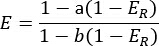
      NOTE: The FRET efficiency (E) reflects the true probability of energy transfer between the donor and acceptor and is independent of the microscope setup, enabling quantitative, reproducible comparisons of FRET measurements across different instruments. The calibration coefficients a and b are instrument-specific and account for donor spectral bleed-through, acceptor direct excitation, and differences in detection response and optical transmission between channels.
   2. To determine these coefficients, acquire calibration images of the reference 5AA and TRAF cell lines as described in Section 2. These constructs have distinct and well-characterized (E_H and E_L, respectively) that serve as calibration points. Time-lapse or z-stack acquisitions are not required; a single image per field is sufficient.
   3. Process the images as described in Section 3.1 to obtain the corresponding FRET indices E_R,H and E_R,L. Then calculate the coefficients using:
      
      
      with c = (E_H - E_L)(1 - E_R,H)(1- E_R,L) where E_H and E_L are the known FRET efficiencies for the 5AA and TRAF constructs, respectively, as previously determined by FLIM from donor fluorescence lifetimes measured in the presence (τ_DA) and absence (τ_D) of the acceptor using the relation  E = 1 - τ_DA/τ_D^37,43. Because FLIM-based FRET measurements rely on donor lifetime rather than fluorescence intensity, this approach is largely insensitive to fluorophore concentration and to variations in experimental settings.
   4. Once these coefficients have been determined for a given microscope configuration, they can be reused to convert any subsequently acquired FRET index E_R into the standardized efficiency E. This calibration ensures that datasets collected on different instruments or with different optical settings are directly comparable. Conversely, if all data to be analyzed originates from the same microscope with identical acquisition parameters, conversion into E is not necessary, and E_R can be used directly for the relative comparison of tension sensor readouts
      NOTE: For accurate calibration, it is recommended to acquire images of the two reference cell lines (5AA and TRAF) within the same acquisition session and under identical exposure, gain, and illumination conditions as used for experimental datasets. Both cell lines should exhibit homogeneous FRET signals within each field of view. If cells display strong intensity variations or saturation, new acquisitions should be performed.
   5. After computing E_R,H and E_R,L, calculate a and b using the formulas given in step 3.4.2. To verify that the calibration is robust:
      1. Check that the computed a and b values are stable across multiple fields of view (variation < 5–10 %).
      2. Confirm that applying these coefficients to recompute E from E_R for the calibration samples yields efficiencies close to their published values (E_H and E_L); deviations greater than 0.02 suggest acquisition or analysis inconsistency.
      3. Optionally repeat the calibration with images acquired on different days to test reproducibility. If variations are observed, consider averaging the a and b coefficients across sessions.
         NOTE: Once validated, the same coefficients can be used for all subsequent conversions, provided the optical configuration (light source type, filter set, camera, and objective) remains unchanged. If any hardware element is modified or settings are substantially adjusted, the calibration should be repeated to ensure quantitative consistency across experiments¹⁵.
5. FRET efficiency (E) to force calibration (pN)
   1. Convert the FRET efficiency values obtained in step 3.1.10 into molecular force using the previously established FRET efficiency-force calibration reported by Grashoff et al.⁴
   2. Estimate the molecular force by fitting the measured FRET efficiencies using the following simplified TSMod calibration equation:
      
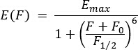
      Here, E_max is the FRET efficiency at 0 pN, F₀ is an empirical scale/offset parameter that defines the effective force range of the transition, and F_1/2 is the characteristic force of the decay. The exponent 6 reflects the expected steep force dependence of FRET arising from Förster theory and the force-induced extension of the flexible polypeptide spacer (the specific 40‑aa repetitive, spider‑silk‑like sequence). Recent work from the Hoffman laboratory has shown that the GPGGA-containing linker used in TSMod behaves as a polymer-like extensible element consistent with worm-like chain modeling, providing a physically grounded description of linker mechanics⁵. In contrast, the present formulation does not aim to provide a more detailed microscopic derivation of TSMod mechanics, but rather to provide a compact, interpretable fit of the calibration curve that captures the force range over which the sensor transitions between high- and low-FRET states. This model, fitted to the Grashoff calibration data and illustrated in Figure 5, is therefore intended as a practical approximation of the calibration relation rather than a full mechanistic reconstruction of TSMod behavior.
      NOTE: In this study, the relationship between FRET efficiency and molecular tension was interpreted using the original linear calibration established for this class of tension sensor by Grashoff et al.⁴. This linear model provides a straightforward mapping between changes in FRET efficiency and changes in applied force and is appropriate when the main objective is to compare relative tension levels between experimental conditions rather than to determine precise absolute force values.
      NOTE: For studies requiring a more rigorous and quantitatively robust calibration of FRET efficiency, more recent frameworks such as QuantiFRET⁴⁴ are recommended. QuantiFRET was developed primarily for sensitized-emission FRET acquired on standard widefield or epifluorescence microscopes, where spectral bleed-through and cross-excitation are the dominant sources of error and typically require a panel of calibration constructs to correct for. The principal advantage of QuantiFRET over a simple linear relationship is that it explicitly accounts for these and other sources of experimental variability within a standardized analysis pipeline. This yields more accurate and reproducible FRET efficiency estimates, improving the reliability of absolute force calibration.
6. Script 2 – FRET_Wound_Healing.py: Band‑based FRET analysis along the wound edge
   This second script is an optional extension specifically developed for wound healing or scratch assays and should be used only when a wound ROI has been defined and spatially resolved analysis along the wound edge is required. It does not replace the main FRET quantification pipeline described above, but provides an additional layer of analysis for experiments focused on collective migration and wound closure. A step-by-step visual guidance of the script is shown in Figure 6.
   1. Use File > Open… to open the script FRET_Wound_Healing.py in Fiji and click Run at the bottom of the script editor window. A dialog box appears prompting the user to select the wound ROI, the FRET image, the band dimensions, and the minimum region size to be removed.
   2. After clicking OK, the script retrieves the image metadata and calibration, then subdivides the wound ROI into a 2D mesh of rectangular sampling bands.
   3. The script performs basic preprocessing and applies a size‑based quality filter to ensure robustness of the measurements. Then it constructs a visual meshing map of the wound region. Each mesh element is filled with the corresponding mean FRET value, producing a spatially segmented map of FRET along the wound. The meshing image is saved as [image_name]_Meshing.tif in the same directory as the FRET image. All generated sampling ROIs are saved as RoiSet_Meshing.zip alongside the meshing image.
   4. The script generates a results table in which:
      1. Each row corresponds to a distance from the wound edge (expressed in µm using the image calibration).
      2. Each column (FRET-line_1, FRET-line_2, etc.) corresponds to one horizontal band line, i.e., one position along the wound edge.
      3.  The table header “Width from WH (microns)” contains the physical distance of each column from the wound edge. The table is displayed in Fiji as “Channel Analysis Results” and exported as WH_Measurements.csv in the same directory.

Resultados

To quantify intramolecular mechanical tension across vinculin at focal adhesions (FAs), a genetically encoded vinculin tension sensor module (VinTS) was used, in which the TSMod FRET-based elastic linker is inserted between the head and tail domains of vinculin, as shown in Figure 1. This design provides a direct, live-cell readout of vinculin conformation and mechanical loading at focal adhesions, enabling in situ monitoring of force transmission at subcellular resolution. To probe the contribution of vinculin autoinhibition and actin binding to force transmission, VinTL, a tail-less control that disrupts force-bearing interactions; VinT12, a constitutively open variant with weakened head–tail autoinhibition; and VinV1001A, a tail-domain mutant with reduced actin binding and altered mechanosensitivity were analyzed (Figure 1). Together, these constructs provide a framework to dissect how vinculin conformation and cytoskeletal coupling shape its mechanical state at focal adhesions, while enabling us to assess how epithelial cell density modulates vinculin tension and how tensile forces are distributed during wound healing.

Effect of cell density on vinculin tension at focal adhesions
To examine how vinculin mechanical loading responds to changes in epithelial cell density, low‑density (LD, <1600 cells/mm²) and high‑density (HD, >1600 cells/mm²) conditions were compared. A representative VinTS-expressing MDCK cell under low-density conditions is shown in Figure 7A, with the donor (mTFP1), acceptor (YFP), and color-coded FRET index images.  These regimes correspond to weak versus strong intercellular contacts and distinct cytoskeletal organizations. In cells expressing VinTS, vinculin tension was strongly modulated by cell density (Figure 7B). At low density, VinTS displayed an intermediate FRET index, consistent with basal, cytoskeleton‑dependent tension at focal adhesions. At high density, the FRET index was significantly lower, indicating increased intramolecular tension across vinculin in crowded epithelial monolayers. This suggests that enhanced cell–cell confinement promotes force transmission through FAs.

In contrast, the VinTL truncation mutant exhibited a uniformly high FRET index under both density conditions, indicative of very low intramolecular tension (Figure 7B). This behavior is consistent with the absence of the tail domain, which prevents actin binding and thereby abolishes force transmission from the actomyosin cytoskeleton to vinculin, explaining the lack of density‑dependent modulation. Conversely, the VinT12 mutant showed a markedly reduced FRET index that remained unchanged across densities, reflecting elevated intramolecular tension (Figure 7B). This result corroborates the auto-activation of VinT12, which remains in an open conformation that favors constitutive engagement with actin and force-bearing adaptor proteins, independent of upstream mechanoregulation. Similarly, the VinV1001A mutant exhibited a higher FRET index than full‑length VinTS under both conditions, indicative of reduced tension (Figure 7B). This behavior is consistent with impaired vinculin–F‑actin binding, which limits force transmission despite preserved focal adhesion localization, thereby preventing sensitivity to changes in cell density.

Together, these results demonstrate that vinculin intramolecular tension is critically influenced by actin binding and adhesion context, whereas vinculin activation and mechanical loading remain separable processes. Tail truncation or defective actin binding results in reduced tension across vinculin, while constitutive opening alters vinculin conformation without implying force transmission through the sensor. Accordingly, cell density modulates vinculin tension only when vinculin retains an intact tail domain and regulated interactions with the actin cytoskeleton, whereas constitutively open or actin-binding-deficient mutants decouple vinculin’s mechanical readout from collective epithelial context.

To provide a quantitative assessment of vinculin loading, we first converted the mean FRET index into FRET efficiency (E) using the calibration established from the control constructs 5AA and TRAF (Figure 7C), according to the linear relation E = a·FRET index+b, with a = 0.064 and b = -0.013 (Section 3.4) This calibration, based on the mean FRET index values measured for these two reference constructs, allowed us to derive a linear conversion and to calculate FRET efficiency for all experimental conditions (Figure 7D). The resulting FRET efficiencies were then projected onto the FRET efficiency–force calibration curve described in section 3.5 and shown in Figure 7E, yielding molecular force estimates in pN. The VinTS construct exhibited a clear reduction of FRET efficiency and, accordingly, an increase in inferred vinculin‑generated forces at high density compared with low density. In contrast, VinTL showed consistently high FRET efficiencies and low inferred forces across conditions, whereas VinT12 and VinV1001A displayed elevated and reduced molecular forces, respectively, in agreement with the qualitative interpretation based on the FRET index. These force‑resolved data confirm that cell‑density‑dependent modulation of vinculin tension requires a structurally intact tail domain and regulated actin binding, and they highlight the quantitative power of the TSMod‑based calibration combined with the simplified physical model introduced in the present work

Vinculin tension distribution during wound healing
Vinculin tension dynamics were also assessed during collective migration using a wound-healing assay, focusing on full-length VinTS. Images were acquired at least 6 h after wounding, when a coherent epithelial sheet had formed and when leader cells were clearly established at the migration front. For each wound-healing condition, initial analysis script was first applied to generate a color-coded FRET index map from the donor and acceptor images (Figure 8A). This map was then further processed using the second script, which averaged FRET index values within 10 × 10-pixel regions of interest to obtain the mean FRET index (%) as a function of distance from the wound edge (Figure 8B). Wound-healing images were analyzed under two conditions: in the absence and in the presence of 0.5 µM cytochalasin D (CytoD), an inhibitor of actin polymerization.

In untreated cells, the FRET index displayed a clear front-to-rear gradient across the migrating sheet. It decreased approximately linearly from the migration front toward the back of the monolayer, with an overall drop of about 3% over 500 µm (Figure 8C). This spatial gradient indicates that vinculin is less tense at the leading edge and progressively more loaded farther from the front. Such a front-to-rear difference has been reported previously in wound-healing contexts²⁹, but unlike these studies, the present analysis captures the full spatial profile over the entire distance to the wound edge. Notably, the FRET values at the front were close to those measured in low-density conditions, whereas values in the back were similar to those observed in high-density monolayers (Figure 7B).

By contrast, CytoD treatment largely abolished the spatial variation in FRET index. Under these conditions, the FRET index remained nearly constant across the wound-healing sheet, at approximately 58%, with at most a very weak spatial trend (Figure 8D). This value is comparable to that observed for the VinTL mutant, which is unable to couple vinculin to the actin cytoskeleton. Together, these observations indicate that the spatial distribution of vinculin tension during collective migration depends on actin polymerization and cytoskeletal coupling, and that the rear of the migrating sheet bears a higher vinculin load than the front under untreated conditions.

These results further emphasize an important point: mechanical forces measured at the molecular scale do not necessarily mirror traction forces measured at the tissue scale. Although traction is often highest at the leading edge of migrating collectives, vinculin tension reflects the force borne by the molecule within focal adhesions, which is shaped not only by global tissue mechanics but also by local molecular engagement, cytoskeletal coupling, and focal adhesion composition. In this sense, vinculin behaves as a mechanosensitive integrator of subcellular force transmission rather than as a simple proxy for macroscopic traction.

Collectively, these data show that vinculin intramolecular tension is spatially patterned during collective migration, with lower tension at the migration front and higher tension in the rear, and that this organization is strongly attenuated when actin dynamics are inhibited.

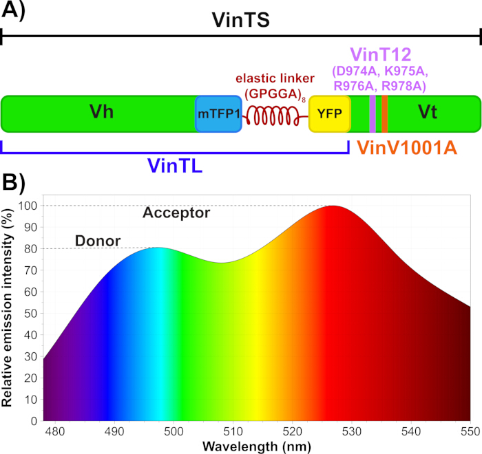
Figure 1: Schematic of the VinTSMod construct and its spectral properties. (A) Schematic representation of the vinculin tension sensor VinTS, in which the TSMod FRET module is inserted between the head and tail domains of vinculin, and of the mutant constructs VinTL, VinT12, and VinV1001A. The TSMod module consists of the donor fluorophore mTFP1 (blue square), the acceptor fluorophore EYFP (yellow square), and elastic linker sequences (GPGGA)₈, represented in red. VinTL is a tail‑truncated, tension‑insensitive control lacking amino acids beyond residue 883. VinT12 carries four charge‑to‑alanine substitutions in the tail domain (D974A:K975A:R976A:R978A) that weaken head–tail autoinhibition. VinV1001A bears a valine‑to‑alanine mutation at residue 1001 that reduces actin binding to the vinculin tail. (B) Spectral emission profile of the TSMod biosensor, showing the donor and acceptor emission peaks used for FRET imaging and quantification. Please click here to view a larger version of this figure.

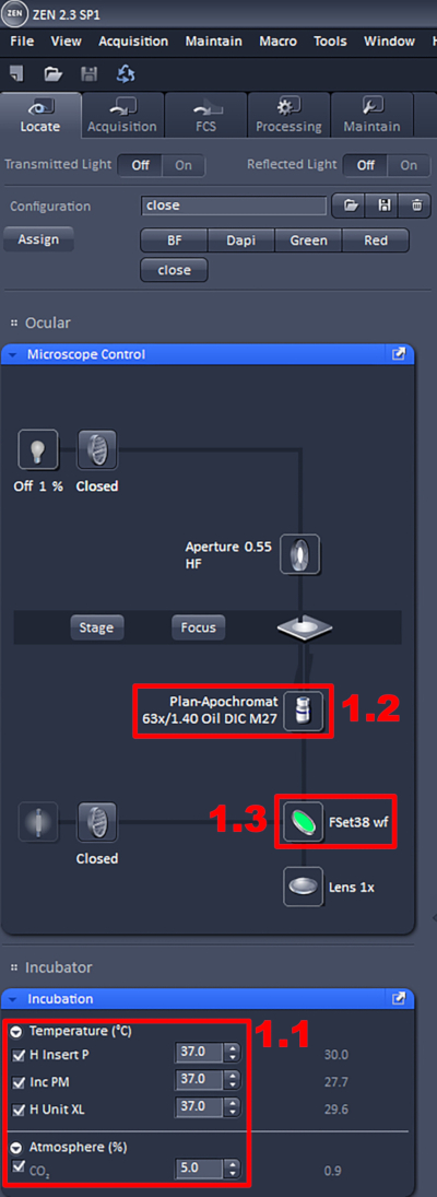
Figure 2: Acquisition panel to visualize fluorescent cells in ZEN software. The ZEN software acquisition panel used for live-cell spectral FRET imaging, showing the environmental control settings, objective selection, and optical configuration for identifying fluorescent cells prior to spectral image acquisition. Please click here to view a larger version of this figure.

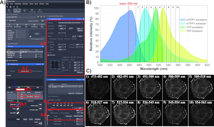
Figure 3: Acquisition panel and spectral sampling settings. (A) Acquisition panel with imaging settings used for spectral confocal imaging in ZEN software. (B) Absorption and emission spectra of mTFP1 and EYFP. The 458 nm excitation line is indicated in red. Black rectangles denote the wavelength bands used to construct the lambda stack, acquired in 8.9 nm increments from 473 to 563 nm, yielding 10 spectral sections. (C) Example of a lambda stack of an MDCK cell expressing VinTS, showing the corresponding wavelength bands indicated in panel B. Please click here to view a larger version of this figure.

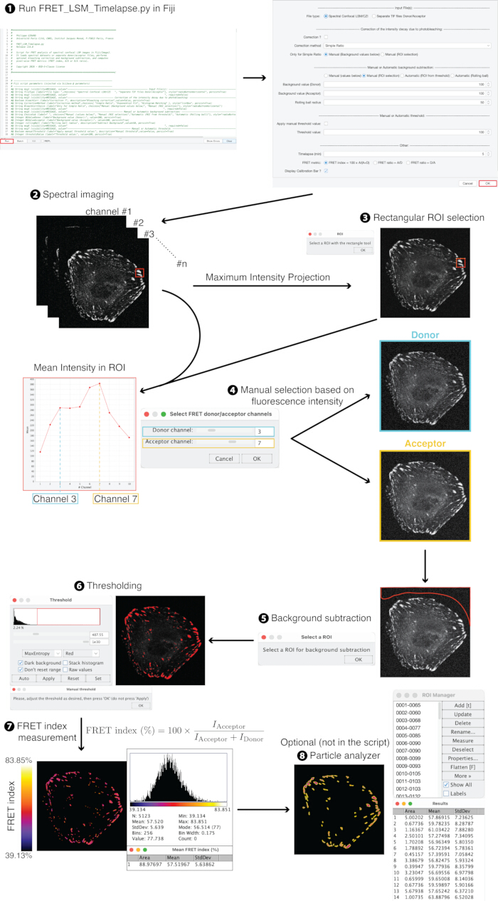
Figure 4: Image analysis workflow of the script FRET_LSM_Timelapse.py. Workflow illustrating the analysis pipeline implemented in the FRET_LSM_Timelapse.py script, including spectral image loading, donor and acceptor channel selection, background subtraction, thresholding, FRET index calculation, and optional focal adhesion-level analysis. Please click here to view a larger version of this figure.

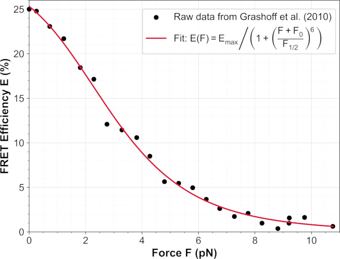
Figure 5: FRET efficiency–force calibration curve for the TSMod‑based vinculin tension sensor. Data points correspond to the calibration values of Grashoff et al.⁴, relating FRET efficiency (E) to applied molecular force (F, in pN). The red line shows the fit of the simplified physical model with E_max = 28%, F₀ = 6.3074 pN and F_1/2 = 9.0923, yielding a coefficient of determination R₂ = 0.9936. Please click here to view a larger version of this figure.

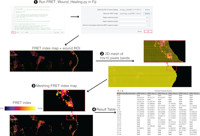
Figure 6: Image analysis workflow of the script FRET_Wound_Healing.py. Workflow illustrating the analysis pipeline implemented in the FRET_Wound_Healing.py script, including wound region selection, generation of the meshing grid, calculation of mean FRET index as a function of distance from the wound edge, and export of quantitative measurements. Please click here to view a larger version of this figure.

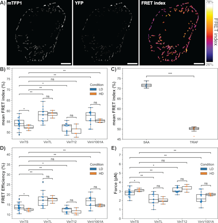
Figure 7: Quantification of vinculin tension by FRET index, FRET efficiency, and force estimation under low- (LD, <1600 cells/mm²) and high-density (HD, >1600 cells/mm²) conditions. (A) Representative image of a VinTS-expressing MDCK cell under low-density (LD) conditions, showing the donor channel (mTFP1), the acceptor channel (YFP), and the corresponding FRET index map (in %), with the associated color bar. Scale bar = 10 µm. (B) Mean FRET index measured for VinTS and the vinculin mutants VinTL, VinT12, and VinV1001A under low- and high-density conditions. (C) Mean FRET index measured for the calibration controls 5AA and TRAF, used to convert FRET index into FRET efficiency in section 3.4 of the protocol according to the linear relation E = a·FRET index + b, with a = 0.064 and b = -0.013. (D) FRET efficiency values calculated for VinTS and the mutant constructs from the calibration established in panel C, shown for LD and HD conditions. (E) Molecular force estimates derived from the FRET efficiency values using the force calibration curve shown in Figure 5, again displayed for LD and HD conditions. Data are presented as mean ± SD from independent experiments. Statistical significance was assessed using a two-sided Mann–Whitney–Wilcoxon test with Bonferroni correction for multiple comparisons. Significance levels are indicated as follows: ns = not significant; *= p < 0.05; **= p < 0.01; ***= p < 0.001. Please click here to view a larger version of this figure.

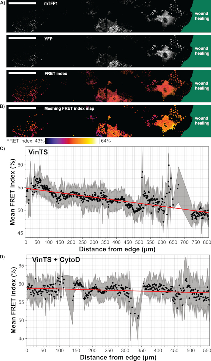
Figure 8: Spatial distribution of vinculin tension during wound healing in VinTS-expressing MDCK cells. (A) Representative wound-healing image showing donor (mTFP1), acceptor (YFP), and color-coded FRET index maps obtained from the first analysis script. The wound edge is highlighted in green. Scale bar = 100 µm. (B) The color-coded FRET map was further processed using the second script, which averaged FRET index values within 10 × 10-pixel regions of interest; the wound edge is also indicated in blue, and the associated color bar is shown. Scale bar = 100 µm. (C,D) Mean FRET index (%) as a function of distance from the wound edge in VinTS-expressing cells, either (C) untreated or (D) treated with 0.5 µM cytochalasin D (CytoD). Data were measured in 10 × 10‑pixel regions of interest across multiple wound healing images. Black markers show the mean FRET index for each distance bin, with gray shaded bands representing the standard deviation. Red lines show linear fits to the data. For untreated cells, the regression equation is y = −0.006615x + 54.837, with a coefficient of determination R²= 0.567, indicating a FRET gradient between the front and the back. For CytoD-treated cells, the regression equation is y = −0.002346x + 58.848 with R²= 0.064, indicating no significant difference in FRET (~58%) between the front and the back after actin polymerization inhibition. Please click here to view a larger version of this figure.

Supplementary Table 1: Published TSMod-based tension biosensors employing spider silk protein (SSP) linkers. Overview of studies using SSP-based TSMod tension biosensors, indicating the FRET fluorophore pair, the targeted mechanosensitive protein, and the experimental model used. Authors shown in bold correspond to the first report of the original construct developed by that laboratory. Please click here to download this file.

Discussão

Genetically encoded, unimolecular FRET biosensors provide a robust and versatile strategy for directly monitoring protein activity and mechanical states in living cells. In this context, the VinTS sensor offers a sensitive readout of intramolecular tension at focal adhesions and junctional structures, enabling mechanical load to be assessed in situ with subcellular resolution. This makes it a powerful framework for probing how cells translate their physical environment into molecular-scale responses.

A major strength of the protocol is that FRET measurements were acquired by spectral imaging on a confocal microscope, using a spectral detector to collect narrow 8.9 nm emission bands centered on the mTFP1 and YFP peaks rather than conventional sensitized-emission FRET on a standard widefield or epifluorescence system. This acquisition strategy substantially reduces spectral bleed-through and cross-excitation between donor and acceptor channels at the detection level, which are major sources of error in classical sensitized-emission FRET and typically require extensive calibration with donor-only and acceptor-only controls. In this context, the low FRET signal observed with the TRAF-based construct should not be interpreted as a loss of signal quality, but rather as its intended role as a deliberately low-FRET reference, used together with the high-FRET 5AA construct to bracket the dynamic range of the sensor, following the strategy of Day et al.³⁷. Because the vinculin tension sensor is intramolecular and maintains a fixed 1:1 donor: acceptor stoichiometry, this two-point bracketing approach is sufficient to convert raw FRET indices into normalized FRET efficiency values without requiring the broader correction-factor framework used for sensitized-emission acquisition.

Several technical considerations are essential for reproducible measurements. In stable cell lines, loss of a fluorophore may occur over time, most likely through recombination events; spectral imaging enables identification and exclusion of such cells from analysis. Importantly, the FRET index is instrument-dependent and cannot be directly compared across different microscopes unless appropriate calibration is performed. Comparisons between constructs or experimental conditions are therefore most robust when performed on the same instrument under stable imaging conditions. This stability can be monitored using FRET standards such as 5AA and TRAF, which consistently provide high and low reference values, respectively³⁷. Although these controls do not need to be included in every experiment, periodic checks remain advisable, particularly after maintenance or at regular intervals, to ensure comparability across datasets.

VinTL, used here as a control, is not biologically inert. As a C-terminal truncation lacking the actin-binding tail domain, it locks vinculin in a constitutively open conformation and may act as a dominant-negative by competing with endogenous vinculin for binding partners and adhesion sites without engaging actin. For this reason, we also included VinV1001A, a point mutant that strongly reduces actin binding while preserving the full-length protein and its autoinhibited conformation. Because it avoids the structural perturbations associated with truncation, VinV1001A provides a more rigorous control and may be preferred in future studies using this sensor. This is consistent with the increasing use of actin-binding-deficient point mutants as vinculin tension sensor controls.

Differences between constructs or conditions can often be appreciated qualitatively in FRET images and quantified by calculating mean FRET values using image analysis tools such as Fiji³⁸. However, statistical testing remains indispensable for determining whether such differences are significant. Beyond statistical significance, interpretation also depends on biological context: variations in FRET index, whether small or large, only become meaningful when compared to a relevant reference state. Converting FRET index values into molecular tension further strengthens interpretation by providing a more intuitive and directly comparable readout³¹.

A further limitation of simplified intramolecular FRET analysis is the potential contribution of mechanically induced fluorescent quenching. Although the fixed 1:1 donor:acceptor stoichiometry of intramolecular sensors such as VinTS has long supported the use of simplified, relative FRET indices rather than fully calibrated FRET efficiency values, recent work from the Hoffman laboratory⁴⁵ showed that mechanical quenching of fluorescent proteins can occur in FRET-based tension sensors, including the vinculin sensor used here, independently of classical FRET. This raises the possibility that part of the measured signal may reflect mechanically induced quenching rather than donor–acceptor separation or orientation alone. Importantly, our conclusions rely exclusively on relative comparisons of FRET index between experimental conditions rather than on absolute FRET efficiency or force values; to this extent, a condition-independent quenching offset would not be expected to alter the qualitative interpretation. However, if the magnitude of mechanical quenching itself scales with mechanical loading, as suggested by Shoyer et al.⁴⁵, this effect could also influence the size of relative FRET differences between conditions subjected to markedly different tension regimes. Therefore, the FRET index measurements were interpreted as a relative readout of vinculin tension dynamics, consistent across independent replicates, while acknowledging that mechanical quenching remains a potential confounding factor that current calibration procedures do not yet fully resolve.

Although developed using the mTFP1/YFP-based TSMod sensor, the image-processing workflow can in principle be adapted to other FRET-compatible fluorophore pairs, such as EGFP/mCherry, Cerulean/Venus, or more recent combinations including Clover-mRuby2⁵ and mNeonGreen/mScarlet-I⁴⁶, provided that appropriate spectral separation and calibration are performed.

The approach is also compatible with multiplex imaging. Several biosensors can now be combined within the same cell, allowing mechanical tension to be examined alongside biochemical signaling. For example, coupling VinTS with kinase activity reporters such as KTR-based sensors^47,48 offers an opportunity to connect force transmission to downstream signaling responses. This requires careful selection of fluorophores to minimize spectral overlap. In practice, the mTFP1/YFP pair can be retained for TSMod, whereas additional reporters can be assigned red-shifted fluorophores such as mRuby2, mKate2, or iRFP713, together with an appropriate nuclear marker when required.

The present study was performed in flat 2D monolayers, and baseline FRET values may differ in 3D environments because of changes in cell morphology, matrix confinement, and adhesion composition. A recent study comparing VinTS in 2D monolayers and 3D multicellular aggregates⁴⁹ reported lower FRET efficiency in 3D, highlighting the influence of microenvironment dimensionality. Direct comparison remains challenging, however, because focal adhesions are difficult to distinguish from intercellular junctions and other interfaces in 3D, and vinculin tension is known to differ between these adhesion types. Accordingly, our 2D measurements provide a useful reference for how cell density and collective migration modulate vinculin tension at focal adhesions, but extrapolation to 3D systems requires caution and context-specific calibration.

Our observation of a front-to-rear gradient in vinculin FRET index during collective migration adds a spatial dimension to this framework. Leader cells at the wound edge displayed a higher FRET index, indicative of a more closed and less loaded vinculin conformation, than cells further back from the migration front. This polarity is consistent with the polarized distribution of traction forces typically observed at the leading edge during wound healing. Recent work further showed that vinculin mechanics at cell-cell adherens junctions are regulated by a phosphorylation-dependent mechanochemical switch at S1033, which controls vinculin loading at these junctions and thereby modulates intercellular friction and the speed and coordination of collectively migrating MDCK monolayers²⁸. Whereas that study focused on biochemical control of vinculin loading at cell-cell junctions, the present results highlight a complementary, spatially resolved aspect of vinculin mechanics across the migrating epithelium. Together, these findings support a model in which vinculin mechanics are regulated both biochemically, through phosphorylation-dependent switches at cell-cell junctions, and spatially, through position-dependent loading across the migration front, suggesting that future studies combining both approaches may further clarify how these regulatory layers are coordinated during collective cell migration.

Although this protocol is presented here in the context of vinculin, it is not restricted to this protein and can be readily adapted to other tension sensors and mechanosensitive systems. TSMod-based biosensors have been extended to a broad range of proteins (Supplementary Table 1). Since the initial development of the vinculin sensor, similar strategies have been successfully extended to proteins involved in cell–cell adhesion (e.g., E-cadherin, VE-cadherin, α-catenin, desmoglein), cytoskeletal organization (e.g., actin, talin, non-muscle myosin II), and nuclear mechanotransduction (e.g., nesprin, lamin A, nuclear envelope proteins). These applications span diverse experimental models, from cultured cells to whole organisms such as C. elegans, Drosophila, and mouse models. Together, they underscore the versatility of TSMod as a modular platform for investigating how mechanical forces are distributed, transmitted, and integrated across biological systems.

Overall, this method provides a robust, accessible framework for quantifying molecular tension in living cells. When combined with appropriate controls, calibration, and statistical analysis, it enables meaningful comparisons across conditions and over time, while also opening the way to integrated studies of mechanical and biochemical signaling.

Materiais

Lista de materiais utilizados neste artigo

Nome	Empresa	Número de catálogo	Comentários
Chemicals, peptides, and recombinant proteins
Cytochalasin D	Sigma-Aldrich	Cat#C8273, CAS Number 22144-77-0
DMEM, low glucose, pyruvate	ThermoFisher	Cat#31885049
DPBS, no calcium, no magnesium	ThermoFisher	Cat#14190144
Fetal Bovine Serum, qualified, heat inactivated, Brazil	ThermoFisher	Cat#10270106
FluoroBrite™ DMEM	ThermoFisher	Cat#A1896701
HEPES (1M)	ThermoFisher	Cat#15630080
L-Glutamine (200 mM)	ThermoFisher	Cat#25030024
Mineral Oil	Sigma-Aldrich	Cat# M5904, CAS Number 8042-47-5
Penicillin-Streptomycin (10,000 U/mL)	ThermoFisher	Cat#15140122
QuikChange II XL Kit	Agilent Technolo- gies	primers: 5’-CCCAGCATGGTAGCTTTCGC TGTGGAAAGAATTTTGA-3’ and 5’- TCAAAATTCTTTCCACAGC GAAAGCTACCATGCTGGG-3’
Trypsin-EDTA (0.5%), no phenol red	ThermoFisher	Cat# 15400054
Experimental models: cell lines
Madin–Darby canine kidney (MDCK) type II G	ECACC	MDCK II (ECACC 00062107)
mTFP1-GPGGA-Venus (5AA)	(Day et al., 2008)	NA
mTFP1-TRAF-Venus (TRAF)	(Day et al., 2008)	NA
Tailless VinculinTS	addgene (gift from Carsten Grashoff)	Plasmid #26020
VinculinTS	addgene (gift from Carsten Grashoff )	Plasmid #26019
Software and algorithms
FIJI with libraries:	(Rueden et al., 2017)	RRID:SCR_002285
FRET_LSM_Timelapse.py	This work	https://github.com/phigirard/FRET
FRET_Wound_Healing.py	This work	https://github.com/phigirard/FRET
Prism VIII software	GraphPad	RRID:SCR_002798
Zen 2011 (Black edition)	Carl Zeiss	RRID:SCR_018163
Other
µ-Slide 8 Well  glass-bottom chambers	Ibidi	Cat#80826
Argon laser -the 458 nm line is optimal for mTFP1 excitation- or equivalent, 25mW	Carl Zeiss	NA
Commercial laser scanning confocal inverted microscope equipped with an incubator	Carl Zeiss	NA
Culture-Insert 2 Well in µ-Dish 35 mm	Ibidi	Cat#81176
Epifluorescence Illuminator HXP 120 V + filter set 38 GFP (EX 470/40).	Carl Zeiss	NA
Main beam splitter 458	Carl Zeiss	NA
Microscope detection: Spectral fluorescence GaAsP array detector.	Carl Zeiss	NA
Microscope objective: 63x/1.4NA Plan-Apochromat oil immersion.	Carl Zeiss	NA
Table-top centrifuge and rotor for 15mL Falcon tubes	generic	NA
Top stage incubator for live cell time lapse imaging (with temperature, humidity, CO2 control)	Carl Zeiss	NA