A Result-Auditable Protocol for Low-Data Classification of Blue-and-White Porcelain Botanical Motifs Using Frozen Chinese-CLIP Features

Resumo

This protocol uses a frozen Chinese vision-language model (Chinese-CLIP) and a linear classifier to classify low-data blue-and-white porcelain botanical motifs with explicit leakage, confounding, and external validity checks.

Resumo

Low-data visual classification is common in cultural heritage documentation, where expert labels are expensive, and image sources are heterogeneous. This protocol provides result-level audit support for classifying five botanical motifs—peony, lotus, chrysanthemum, plum blossom, and bamboo—on blue-and-white porcelain. It combines operational label definitions, source documentation, perceptual hash screening, and fixed, stratified, image-level splits with a frozen Chinese Contrastive Language–Image Pre-training (Chinese-CLIP) Vision Transformer (ViT-L/14-336) visual encoder. A training-only StandardScaler and an L2-regularized multinomial logistic regression classifier form the primary model. In a 259-image demonstration, five overlapping image-level splits yielded 91.28% ± 2.47% accuracy and 91.22% ± 2.44% macro-F1. These are image-level demonstration estimates and may be optimistic because complete artifact identifiers are unavailable; they should not be interpreted as artifact-level, population-level, or confirmatory performance. A retrospective sensitivity analysis that excluded training images linked to test images at a perceptual hash distance ≤15 yielded 91.03% ± 2.03% accuracy. The protocol also specifies few-shot evaluation, metadata controls, feature baselines, prompt sensitivity, and checksum-based archiving. An exploratory assessment of all 60 external images yielded 85.00% accuracy and 85.89% macro-F1 against provisional labels, and 83.33% accuracy and 84.31% macro-F1 against labels from one blinded professor. Six label disagreements remain unadjudicated. A 54-image agreement subset is secondary only. Because the external v2 collection included replacements after model errors were inspected, none of these external results constitutes independent confirmatory validation. The workflow supports expert-reviewed candidate labeling and retrieval, not autonomous attribution, dating, or authentication.

Introdução

In 2024, museums across China received 1.49 billion visits, while the national cultural relics policy calls for digital resource databases, high-resolution collection data, open sharing, and technology-led protection workflows^1,2. Ceramic histories and motif references document the chronological and stylistic significance of botanical decoration on blue-and-white porcelain^3,4,5; once such motifs are isolated as image crops, their variation poses an operational challenge for classification. Cultural-heritage artificial intelligence now includes museum-exhibit understanding and museum toolkits^6,7,8,9, broad machine-learning applications and automated pottery or porcelain analysis^{10,11,12,13,14,15,16}, and heritage image classification or detection^17,18,19. Earlier visual pipelines range from handcrafted local descriptors to ImageNet-pretrained convolutional neural networks^20,21.

Frozen representation models reduce the number of task-specific parameters that must be estimated from a small labeled set. DINOv2, Contrastive Language–Image Pre-training (CLIP), and Chinese Contrastive Language–Image Pre-training (Chinese-CLIP) provide self-supervised or vision-language representations^22,23,24, while transfer-learning, few-shot, and linear-probe studies provide the methodological basis for evaluating whether a fixed representation is readable by a simple classifier^{19,25,26,27,28}. Fine-tuning addresses a different question and can distort pretrained features or reduce out-of-distribution robustness²⁹, whereas prompt learning and adapter methods introduce additional task-specific choices^30,31,32.

Small datasets introduce distinctive validity threats. Perceptual-hash (pHash) screening can identify highly similar files³³, but image-level random splits still require caution when artifact or plate identifiers are incomplete, and group-disjoint validation is preferable when grouping information exists^34,35. Representation plots and retrieval examples are diagnostic rather than causal explanations: Grad-CAM localizes responses³⁶, while attention-flow methods and the debate over whether attention constitutes explanation show why visualization must not be equated with faithful attribution^37,38,39. Uniform Manifold Approximation and Projection (UMAP) is therefore used only to describe embedding geometry⁴⁰.

The primary demonstration uses 259 Portable Network Graphics (PNG) motif crops divided among peony (n = 50), lotus (n = 54), chrysanthemum (n = 51), plum blossom (n = 52), and bamboo (n = 52). The dataset composition is summarized in Table 1, and the operational definitions of the five motif classes are provided in Table 2. Most images were derived from a published ceramic catalog, with a smaller museum-web component and one image with unknown source metadata. Two domain-informed annotators independently assigned internal motif labels and resolved disagreements by discussion. Source, dynasty, and image identifiers are retained so that confounding and external validity limitations remain visible.

This article converts that study into a result-auditable method. It specifies the primary frozen Chinese-CLIP linear probe, comparisons with DINOv2 classification-token (CLS) features and ResNet50, nested few-shot subsets, a metadata-only control, prompt sensitivity, and an exploratory external assessment applied without retuning. The audit package supports numerical verification from retained identifiers, features, predictions, hashes, and checksums; it does not recreate image preprocessing, feature extraction, pHash generation, or fine-tuning from the original pixels. The complete workflow is summarized in Figure 1.

Protocolo

1. Software environment and verification scope

1. Run downstream verification using a recorded environment. To match the R4 analyses, use Python 3.14.4 and the measured software versions provided in Supplementary File 1.
2. Use Supplementary File 2 for prospective method scripts and Supplementary File 3 for archived command-line illustrations. Use source images only under their applicable publisher or museum conditions.
   NOTE: The R4 analyses were executed locally with Python 3.14.4. The historical Python 3.12 environment definitions are retained separately and were not tested in containers during the revision. Historical feature extraction and exploratory fine-tuning used Device A. The supplied result-verification package is image-free because source-image rights remain with the respective monograph publisher and museum collections. It supports auditing from retained derived data but does not regenerate features or hashes from pixels. Any source image proposed for publication must be supported by documented permission or compliance with the applicable rights-holder terms; otherwise, use only author-created diagrams and non-reconstructive derived results.

2. Prepare the image dataset and documentation

1. Create one record per motif crop with a stable image_id, motif_class, source_type, source_reference, dynasty, width, height, file format, and rights status.
2. Restrict the target vocabulary before inspecting model outputs. Use the five operational classes: peony, lotus, chrysanthemum, plum blossom, and bamboo for this demonstration.
   1. Assign peony when the motif shows multiple overlapping petal layers, a full, rounded corolla, and broad or lobed leaves; flag chrysanthemum as the principal confusion.
   2. Assign chrysanthemum when elongated or curled petals radiate from a dense center; flag peony as the principal confusion.
   3. Assign lotus when broad petals form a rosette and seedpods, lotus leaves, or an aquatic composition are present; flag peony when those context cues are absent.
   4. Assign plum blossom when small five-petaled flowers occur on slender angular branches, and assign bamboo when segmented culms and narrow lanceolate leaves dominate.
3. Have two domain-informed annotators label images independently before model training. Resolve disagreements through discussion or a pre-specified adjudicator, and retain the pre-resolution labels when possible.
4. Exclude images whose principal motif is outside the vocabulary, too incomplete for expert judgment, heavily obscured, or below the resolution needed to distinguish diagnostic structure. Do not exclude difficult but interpretable examples after viewing predictions.
5. Record the rights holder and applicable use conditions for every source image. Do not place catalog or museum pixels in a public artifact unless permission or the relevant rights statement allows redistribution. The verification package must contain only identifiers and non-reconstructive derived data.

3. Configure the software environment

1. Copy the supplied result-verification package to a new working directory. Preserve its directory structure and do not edit the archived CSV files before verification.
2. Create and activate an isolated environment. To match the measured revision run, use Python 3.14.4 and requirements_revision_tested.txt; retain a separate record if another runtime is used.
   1. Run “python -m venv .venv”, then activate it with the command appropriate for the operating system.
3. Install the measured revision dependencies with "python -m pip install -r 10_software_and_model_configuration/requirements_revision_tested.txt" from Supplementary File 1.
   NOTE: The earlier requirements_verification.txt and Docker/Conda definitions are candidate historical environments, not tested R4 containers.
4. For prospective feature re-extraction, use the documented environment and scripts in Supplementary File 2. Cache the required model weights locally before a disconnected or archival run.
5. Record the operating system, central processing unit (CPU) or graphics processing unit (GPU), Python version, package versions, model identifier, model revision or weight digest, and random seeds. Treat differences in Basic Linear Algebra Subprograms (BLAS) and solver implementations as possible sources of boundary-level numerical variation.

4. Standardize and inspect the motif crops

1. Store each crop as PNG or another lossless format under its stable image_id. Do not encode the motif class in any path accessible to the data loader.
2. Convert red–green–blue–alpha (RGBA) images to red–green–blue (RGB) against a documented neutral background. Inspect transparency, color channels, orientation, severe compression, crop completeness, and duplicate identifiers.
3. Retain original crop dimensions in the metadata.
   NOTE: In the demonstration,crop widths ranged from 238 to1748 pixels,and crop heights ranged from 224 to 2112 pixels.
4. Apply the preprocessing function paired with each pretrained encoder. For Chinese-CLIP ViT-L/14-336, resize and center-crop to 336 x 336 pixels and use the model-specific normalization. Do not create distinct preprocessing settings for test images.
5. Perform a blinded spot-check of at least five images per class after preprocessing. Confirm that the central motif remains visible and that center cropping has not removed decisive branch, leaf, petal, or culm features.

5. Audit near-duplicates and create fixed splits

1. Calculate a 64-bit perceptual hash (pHash) for every image and compute the Hamming distance for every unordered image pair. For a new prospective dataset, record the exact library, function, version, hash size, color conversion, and preprocessing.
   NOTE: The historical demonstration retains the 64-bit hashes but not the original hash-generation implementation. Do not substitute a later library for the archived implementation; the prospective ImageHash example in Supplementary File 2 is explicitly separate.
2. Flag every pair with Hamming distance ≤8 as a near-duplicate candidate. Additionally, enumerate train–test pairs at distance ≤15 for every fixed split, recording both all-class and same-class counts. Document the reviewer, date, evidence, and uncertainty for any visual assessment; distinguish human review from AI-assisted inspection.
   NOTE: No pair met the historical ≤8 threshold. Same-class cross-split counts at ≤15 were 2, 5, 6, 8, and 6 for seeds 42, 123, 456, 789, and 2024, respectively: 27 pair–split records representing 11 unique pairs. Historical human-review records cover only the two seed = 42 pairs. During revision, all 11 unique pairs underwent AI-assisted visual inspection and byte- and pixel-equality checks. This additional inspection is not an independent human adjudication and does not establish artifact or plate identity.
3. Group confirmed duplicate files, duplicate published plates, or known multiple crops of the same physical object before partitioning, and place the group wholly in training or test data. Because complete artifact and plate identifiers were unavailable for the demonstration, the pHash audit reduces detectable file-level leakage but does not establish artifact-disjoint validation^34,35. Accordingly, the reported internal metrics may be optimistic and should be treated as image-level estimates given incomplete artifact metadata.
4. Generate five fixed 70/30 image-level splits with train_test_split(test_size=0.30, stratify=y, random_state=seed) using seeds 42, 123, 456, 789, and 2024.
5. Save train and test image_id values for every split. For the 259-image demonstration, verify that each split contains 181 training and 78 test images and that all five classes appear in both partitions.
6. Freeze the split files before fitting classifiers or comparing prompts. Calculate and archive a Secure Hash Algorithm 256-bit (SHA-256) checksum for each split file.
7. As a retrospective sensitivity analysis, identify every training image linked directly to any fixed test image at pHash distance ≤15, irrespective of class. Remove those training images only; preserve the 78 test images, labels, features, and classifier settings in each split. Refit the scaler and classifier on the remaining training images, and compare predictions with an unchanged-split refit in the same runtime.
8. Use 11_verification_scripts/analyze_revision_sensitivity.py and retain all outputs in folder 12_revision_analyses of Supplementary File 1.
   NOTE: The threshold was inherited from an earlier sensitivity screen.This retrospective sensitivity analysis was not preregistered and does not replace artifact-grouped validation.

6. Extract frozen Chinese-CLIP image features

1. Load the Chinese-CLIP checkpoint “AI-ModelScope/chinese-clip-vit-large-patch14-336px,” using the archived model identifier. Place the model in evaluation mode, freeze all encoder parameters, and disable gradient computation for the primary feature extraction.
   NOTE: The checkpoint is based on the Chinese-CLIP model family²⁴. It uses a ViT-L/14 visual encoder from the Vision Transformer family⁴¹.
2. Encode every preprocessed RGB crop once with the visual encoder. Extract the 768-dimensional image vector and L2-normalize each vector.
3. Save one row per image in a numeric feature file keyed by image_id. Verify that the identifier order exactly matches the metadata index and that all feature values are finite.
4. Check that every normalized feature vector has Euclidean norm close to 1.0 within floating-point tolerance. Re-extract any missing, nonfinite, or zero-norm row.
5. Record the exact model identifier and revision. Do not silently replace the model with another Chinese-CLIP size or input resolution, because feature dimensionality and performance will change.

7. Fit and evaluate the primary linear probe

1. For each fixed split, select training and test feature rows by image_id. Assert that the two identifier sets are disjoint and that no test row enters model fitting.
2. Fit StandardScaler only on the training features, then transform the training and test matrices with that fitted scaler.
3. Fit L2-regularized logistic regression with C = 1.0, solver = “lbfgs”, max_iter = 2000, and the five class labels. Do not tune C or any preprocessing choice on a test partition.
4. Predict every test image and export image_id, true label, predicted label, split seed, and method. Retain probabilities or decision scores when the software version consistently exposes them.
5. Calculate accuracy and macro-F1 for each split, then report the mean and sample standard deviation across the five splits. Also, retain a confusion matrix and class-specific precision, recall, and F1 for a representative prespecified split.
6. Confirm that the demonstration output is approximately 91.28% ± 2.47% accuracy and 91.22% ± 2.44% macro-F1. If accuracy differs materially, inspect the alignment of identifiers, feature normalization, training-only scaling, class order, and split files before changing model settings.

8. Run comparisons, sample-efficiency analyses, prompts, and validity controls

1. Construct 1-, 2-, 4-, 8-, 16-, and 32-shot subsets inside each outer training partition while keeping the outer test partition fixed. Use the archived nested subset indices and never draw k-shot examples from a test set.
2. Refit the scaler and classifier from scratch on each k-shot subset. Repeat subset sampling three times within each outer split when enough images are available, average within split, and then summarize across the five outer splits.
3. Fit frozen DINOv2 CLS and ResNet50 logistic-regression (LogReg) baselines on the same fixed splits and k-shot indices. Use encoder-specific preprocessing, L2-normalize the exported features, and fit StandardScaler only on the corresponding training rows.
4. For Chinese-CLIP + DINOv2 fusion, normalize the 768-dimensional Chinese-CLIP vector and 1024-dimensional DINOv2 CLS vector separately, concatenate them into a 1792-dimensional vector, and fit the same training-only StandardScaler and logistic regression (C = 1.0, solver = “lbfgs,” max_iter = 2000) on each split.
5. For prototype matching, compute one class prototype from only the current split’s L2-normalized Chinese-CLIP training vectors, renormalize each mean prototype, and assign each test image to the class with the highest cosine similarity. Do not use test images when forming prototypes.
6. For the archived exploratory fine-tuning comparison, unfreeze only vision_model.encoder.layers[22:24] and keep post_layernorm and all other encoder parameters frozen. Attach a Linear(768, 5) training head and optimize cross-entropy with AdamW (learning rate 1 x 10⁻⁴; weight decay 0.01), CosineAnnealingLR (T_max = 10), batch size 4, and 10 epochs. Re-extract 768-dimensional features after training, then evaluate them with a training-only StandardScaler and logistic regression (C = 1.0, solver = "lbfgs", max_iter = 2000).
7. Select the archived fine-tuning configuration only within the seed = 42 training partition: stratify 20% of its 181 images as an inner validation subset, and compare learning rate ∈ {1 x 10⁻⁵, 5 x 10⁻⁵, 1 x 10⁻⁴}, epochs ∈ {5, 10}, and unfreezing ∈ {last 1, 2, or 4 blocks}. Run the selected configuration once per outer split, and label this comparison as exploratory in all outputs.
   NOTE: No separate augmentation pipeline, framework random seed, checkpoint-selection rule, or original training script was retained. The result is therefore an archived exploratory audit rather than an independently pixel-level reproducible protocol.
8. Fit a metadata-only baseline using one-hot encoded dynasty and image-source categories. Fit the encoder only to training metadata and map missing or unseen levels to “Unknown.” Treat strong metadata performance as a confounding warning, not as a deployable image classifier.
9. Construct motif class x dynasty and motif class x image-source contingency tables after excluding the one bamboo image with both fields missing. Report Pearson χ², degrees of freedom, asymptotic p, and Cramér’s V. Because expected counts below five occur, use fixed-margin Monte Carlo sampling as the primary inference (1,000,000 draws; seed = 42; SciPy 1.17.1).
10. Evaluate the concise Chinese class-name prompt and the 25 designed semantic prompts (DSPs) only as secondary sensitivity analyses. L2-normalize text vectors; for the DSP ensemble, average the five prompt vectors within each class and renormalize the class prototype; classify by cosine similarity. Report only the concise class-name and DSP-ensemble conditions retained in the result-verification package. Use the exact UTF-8 Chinese strings in Supplementary File 4.
    NOTE: The accompanying English translations are provided for review only and were not used for text encoding.
11. Apply UMAP to all 259 feature vectors using n_neighbors = 15, min_dist = 0.1, metric = “cosine,” and random_state = 42. Use the two-dimensional projections only as qualitative descriptions of embedding geometry.
12. For nearest-neighbor retrieval, use the seed = 42 split, 78 test queries, and the corresponding 181-image training library. L2-normalize features, rank candidates by cosine similarity, exclude the query from any candidate library in which it occurs, and resolve ties stably by candidate index. Define Hit@k as the percentage of queries for which at least one of the k nearest training images has the same motif label; report Hit@1 and Hit@5, and do not treat retrieval or UMAP as a faithful explanation of the logistic-regression decision function.

9. Assess the external collection without retuning

1. For a new confirmatory study, lock external inclusion criteria, images, labels, and analysis rules before examining model predictions. Retain collection, object URL, or accession, crop provenance, label records, rights status, and selection history. The historical v2 demonstration deviated from this requirement and must remain exploratory.
   NOTE: In the demonstration, retained source records link 56 of 60 images to five named collections: the Victoria and Albert Museum (n = 39), the Metropolitan Museum of Art (n = 12), the Cleveland Museum of Art (n = 2), the Ethnological Museum in Berlin (n = 2), and the Shanghai Museum (n = 1). Four images have no retained source record.
2. For a new study, obtain independent labels and define a disagreement-resolution rule before scoring. In the historical demonstration, one professor at Jingdezhen Ceramic University reviewed all 60 provisional labels while blinded to model predictions; no second independent expert or third-party adjudication was available. Retain both label records unchanged.
3. After completing internal validation, refit StandardScaler and the logistic-regression classifier once using all 259 internal image features under the unchanged C = 1.0, solver = "lbfgs", and max_iter = 2000 configuration. Freeze the fitted scaler and classifier, then apply them to the 60 external image features without further training, threshold adjustment, prompt revision, or class-specific correction.
   NOTE: This is an exploratory assessment, not confirmatory validation.
4. Treat the complete 60-image collection as the primary exploratory external analysis and report results separately against the provisional labels and the blinded-reviewer labels.
   NOTE: Neither label set is an adjudicated gold standard.
5. Retain the 54-image reviewer–provisional agreement subset only as a secondary sensitivity analysis, and report its six excluded disagreements explicitly.
   NOTE: The six disagreements comprise five provisionally labeled chrysanthemum images and one provisionally labeled peony image.
6. Calculate accuracy, macro-F1, and class-specific F1 on all 60 images against both label records. Verify 51 of 60 provisional-label predictions (85.00% accuracy; 85.89% macro-F1) and 50 of 60 reviewer-label predictions (83.33% accuracy; 84.31% macro-F1). Report the 54-image agreement-subset result separately as a sensitivity analysis: 48 of 54 correct, 88.89% accuracy, and 90.01% macro-F1.
7. Retain the dataset-version limitation, and treat the external result as exploratory evidence across collections rather than as a preregistered or confirmatory benchmark.
   NOTE: The supplied external working record identifies v2 as post-error-analysis and includes replacements made after model errors were inspected.

10. Verify, archive, and define the decision boundary

1. Run “python 11_verification_scripts/verify_all_results.py” from the root of the unmodified result-verification package.
2. Require successful checksum, identifier, split, prediction, summary, few-shot, metadata, pHash, prompt, retrieval, configuration, and fine-tuning aggregation checks. Investigate any failure before regenerating an archived output.
3. If a refit differs only at a numerical decision boundary, compare image_id-level predictions and metrics. Record the software stack, the affected identifier, and whether accuracy or conclusions changed; preserve the originally archived outputs alongside the rerun report.
4. Package metadata, features, split indices, predictions, summaries, prompts, scripts, configuration files, and SHA-256 checksums. Exclude copyrighted images unless redistribution is explicitly permitted.
5. Use the classifier only to propose candidate motif labels or retrieve similar images for expert review. Do not use model output alone for artist attribution, dating, authentication, valuation, conservation intervention, or legal/cultural-property decisions.

Resultados

Inspection of all 11 unique same-class candidate pairs included exact byte and decoded-pixel comparisons, AI-assisted visual  inspection,and review by one blinded externa lexpert. The expert found no clear same-object, same-publication-plate, or related-crop linkage; the review is exploratory and does not establish artifact-level independence or inter-rater reliability. Several pairs share decorative structure, but their physical-object identity remains unresolved.

To assess sensitivity without assuming that unresolved candidates were independent, all training images directly linked to a test image by pHash distance ≤15 were excluded, regardless of class. This removed 16, 17, 22, 16, and 21 training images, leaving 165, 164, 159, 165, and 160 per split while preserving all 78 test queries. Mean accuracy was 91.03% ± 2.03% and macro-F1 was 90.94% ± 2.00%, compared with 91.28% ± 2.47% and 91.20% ± 2.47% for unchanged-split refits in the same runtime. The archived primary macro-F1 was 91.22% ± 2.44%; its small difference from the same-runtime refit reflects the recorded seed = 789 numerical boundary case. The observed mean changes of −0.26 percentage point in both accuracy and macro-F1 are descriptive, not evidence of statistical equivalence or artifact-disjoint performance. Supplementary Table 1 reports all five splits, with exclusions and per-image predictions in Supplementary File 1.

The primary output is an image-level performance estimate for a small trainable head. Across five fixed image-level splits, Chinese-CLIP plus logistic regression produces 91.28% ± 2.47% accuracy and 91.22% ± 2.44% macro-F1. In the representative seed = 42 split, 72 of 78 images are correct (92.31% accuracy; 92.25% macro-F1). The six errors are distributed across several one-image confusion paths rather than a complete collapse of one class. Inspecting these errors should guide annotation review and interface design, but it must not be used to retroactively relabel the test set. Per-seed values are reported in Supplementary Table 2.

Frozen representation choice matters. Chinese-CLIP linear probing outperforms DINOv2 CLS plus logistic regression (84.62% ± 4.15% accuracy) and ResNet50 plus logistic regression (75.64% ± 4.53% accuracy). Concatenating Chinese-CLIP and DINOv2 features does not improve the primary result (90.51% ± 2.50%), showing that a larger feature vector and a second encoder need not provide complementary information. Last-two-block fine-tuning reaches 95.13% ± 1.90% but updates approximately 25 million parameters, compared with 3,845 trainable parameters for the linear probe. This exploratory gain must be weighed against optimization sensitivity, computational cost, and the risk of overfitting. The full comparison is summarized in Table 3 and Supplementary Table 2.

Figure 2 and Table 4 present the few-shot learning curves, which describe sample efficiency within the archived image-level partitions. Chinese-CLIP linear probing rises from 38.0% ± 3.7% at one image per class to 75.0% ± 3.9% at eight images per class, 85.0% ± 1.8% at 16 images per class, and 90.1% ± 2.3% at 32 images per class. DINOv2 is similar at one-shot but falls behind from two-shot onward; ResNet50 remains lower throughout. For reruns of the same retained data, a large discrepancy warrants checking identifier alignment, feature files, and training-only scaling. A new collection may perform differently because of domain shift and should not be expected to match these values.

Secondary controls define what the successful classifier does not establish. The metadata-only baseline reaches 27.44% ± 3.46% accuracy and 21.96% ± 3.86% macro-F1. Source is associated with motif class (χ² = 34.420, df = 4, p < 0.001, Cramér’s V = 0.365). The dynasty association is borderline and sensitive to the inferential method: fixed-margin Monte Carlo p = 0.048745, whereas the asymptotic p = 0.050737 (χ² = 15.463, df = 8, Cramér’s V = 0.173). Concise Chinese prompts achieve 81.03% ± 2.29% zero-shot accuracy, the DSP ensemble achieves 78.97% ± 4.21%, and prototype matching achieves 77.18% ± 6.62%. These controls are diagnostic and do not replace the primary visual classifier. The metadata analyses are presented in Supplementary Table 3, retrieval metrics are reported in Supplementary Table 4, and prompt sensitivity is presented in Supplementary Table 5. Supplementary Figure 1 shows the qualitative embedding projections, and identifier-only retrieval examples are shown in Supplementary Figure 2.

The complete 60-image external collection is the primary exploratory analysis; no population-level or confirmatory inference is intended. One professor at Jingdezhen Ceramic University reviewed labels while blinded to model predictions. The classifier was refitted once on all 259 internal images and applied unchanged to all 60 external features. Against provisional labels, 51 of 60 predictions were correct (85.00% accuracy; 85.89% macro-F1). Against blinded-reviewer labels, 50 of 60 were correct (83.33% accuracy; 84.31% macro-F1). Reviewer and provisional labels agreed for 54 images; the six disagreements—five provisional chrysanthemum labels and one provisional peony label—were not adjudicated by a third reviewer. The 54-image agreement subset yielded 48 correct predictions (88.89% accuracy; 90.01% macro-F1) and is reported only as a secondary sensitivity analysis. This analysis hierarchy was changed during revision in response to selection-bias concerns; it was not prespecified. The retained v2 selection history records replacements made after model errors were inspected, so all external results are exploratory and do not constitute independent confirmatory validation. Figure 3 and Table 5 report the internal and external confusion structure and class-level results.

The result-verification package provides a static SHA-256 manifest and tolerance-aware checks. A local R4 run completed the archived result checks and the new revision checks; the measured software versions and execution record are included in Supplementary File 1. This does not establish successful execution of Docker/Conda or pixel-to-result reconstruction. The verifier recalculates aggregate metrics from retained predictions and checks supported classifier refits. Few-shot and fine-tuning checks use retained outputs rather than retraining. In the unchanged primary refit, one seed = 789 prediction for INT_0214 changes from one incorrect class to another; accuracy remains 88.46%, while macro-F1 changes from 88.37% to approximately 88.26%. Baseline refit differences are retained in the report rather than silently replacing archived predictions. Table 6 summarizes checkpoints.

Data Availability:

The image-free result-verification package is provided as Supplementary File 1 and deposited on Zenodo as a versioned public record (https://doi.org/10.5281/zenodo.22872797). The package contains de-identified internal and external image indices, five fixed train-test splits, per-image predictions, per-seed summaries, few-shot outputs, metadata contingency counts, and baseline outputs, retained 64-bit pHash values and distance audits, the 25 Chinese-designed semantic prompts, extracted feature arrays, software and model configuration records, prospective verification scripts, Dockerfile, Conda environment definition, retrospective external-label analyses, the pHash candidate-exclusion sensitivity analysis, the de-identified summary of the 11-pair blinded expert review, and SHA-256 checksums. The package supports result-level verification and classifier refitting from retained derived data, but it does not reproduce pixel-level preprocessing, feature extraction, historical pHash generation, or exploratory fine-tuning from source pixels. Original catalog and museum images are not redistributed because of copyright and reuse restrictions. 

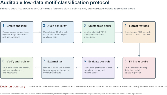
Figure 1: Result: an auditable low-data motif-classification protocol. The workflow separates dataset curation, pHash screening, fixed partitions, frozen feature extraction, training-only scaling, linear probing, validity controls, external testing, and checksum-based archiving. Because source pixels are excluded from the shared package and the historical pHash generator is unavailable, the workflow supports audit from retained derived data rather than full pixel-to-result regeneration. pHash, perceptual hash. Please click here to view a larger version of this figure.

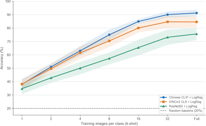
Figure 2: Few-shot learning curves for frozen Chinese-CLIP, DINOv2 classification-token (CLS), and ResNet50 representations. Points show mean accuracy across five fixed outer splits; shaded bands show sample standard deviation. For 1–32 shots per class, values are first averaged across three nested subset samples within each outer split. Full uses 181 training images per split. LogReg, logistic regression. Please click here to view a larger version of this figure.

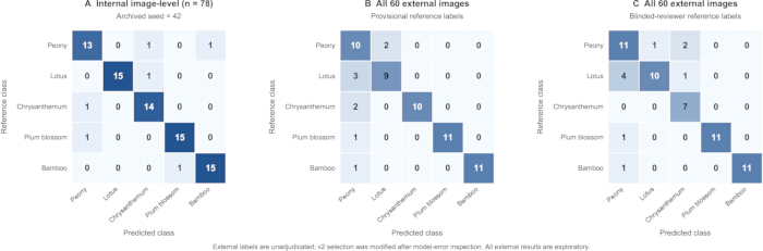
Figure 3: Internal and exploratory external confusion matrices. (A) The archived internal seed-42 split (n = 78). (B) External confusion matrix against provisional labels. (C) External confusion matrix against blinded-reviewer labels. Rows are reference labels and columns are predictions. Neither external label set is an adjudicated gold standard. The external v2 selection history includes post-error-analysis replacements. The 54-image agreement-subset sensitivity result appears in Table 5 and Supplementary File 1. Please click here to view a larger version of this figure.

Motif class	Total	Catalog	Museum	Unknown source	Yuan	Ming	Qing	Unknown dynasty
Peony	50	49	1	0	6	21	23	0
Lotus	54	53	1	0	6	31	17	0
Chrysanthemum	51	43	8	0	5	33	13	0
Plum blossom	52	52	0	0	1	32	19	0
Bamboo	52	37	14	1	1	25	25	1
Total	259	234	24	1	19	142	97	1

Table 1: Dataset composition of the internal image set. Distribution of the 259 internal images by motif class, image source, and dynasty. One bamboo image has unknown source and dynasty metadata.

Motif class	Principal diagnostic attributes	Potentially confusable class
Peony	Multiple overlapping petal layers; full, rounded corolla; broad, often lobed leaves.	Chrysanthemum
Chrysanthemum	Dense center with elongated petals radiating outward; often flat or hemispherical.	Peony
Lotus	Broad petals arranged as a rosette; may include seedpods, lotus leaves, or aquatic composition.	Peony
Plum blossom	Small five-petaled flowers on slender, angular branches; clear spacing between blossoms.	—
Bamboo	Segmented culms and branches with narrow, lanceolate leaves, often in clusters.	—

Table 2: Operational definitions of the five motif classes. Principal diagnostic attributes used to distinguish peony, chrysanthemum, lotus, plum blossom, and bamboo motifs, with potentially confusable classes indicated where applicable.

Method	Accuracy, mean ± SD (%)	Macro-F1, mean ± SD (%)
Chinese-CLIP + LogReg	91.28 ± 2.47	91.22 ± 2.44
Last-two-block fine-tuning (exploratory)	95.13 ± 1.90	95.07 ± 1.91
Chinese-CLIP + DINOv2 + LogReg	90.51 ± 2.50	90.32 ± 2.52
DINOv2 CLS + LogReg	84.62 ± 4.15	84.18 ± 4.00
ResNet50 + LogReg	75.64 ± 4.53	75.58 ± 4.64
Chinese-CLIP prototype matching	77.18 ± 6.62	77.05 ± 6.62
Chinese-CLIP zero-shot (concise)	81.03 ± 2.29	80.16 ± 2.36
Chinese-CLIP zero-shot (DSP ensemble)	78.97 ± 4.21	78.07 ± 4.70
Metadata-only LogReg (dynasty + source)	27.44 ± 3.46	21.96 ± 3.86

Table 3: Classification performance of the evaluated methods. Accuracy and macro-F1 are reported as mean ± sample standard deviation across five fixed, overlapping image-level splits. The last-two-block fine-tuning analysis was exploratory. LogReg, logistic regression; CLS, classification-token feature; DSP, designed semantic prompts.

Shots per class	Training n	Chinese-CLIP + LogReg	DINOv2 CLS + LogReg	ResNet50 + LogReg
1-shot	5	38.0 ± 3.7	38.2 ± 4.0	34.7 ± 4.0
2-shot	10	51.0 ± 2.6	49.7 ± 3.4	42.8 ± 3.7
4-shot	20	63.0 ± 3.5	61.5 ± 4.6	50.1 ± 4.6
8-shot	40	75.0 ± 3.9	70.4 ± 4.6	57.4 ± 4.4
16-shot	80	85.0 ± 1.8	80.1 ± 3.3	65.5 ± 5.9
32-shot	160	90.1 ± 2.3	84.7 ± 4.5	73.2 ± 5.7
Full	181	91.28 ± 2.47	84.62 ± 4.15	75.64 ± 4.53

Table 4: Few-shot classification performance of frozen visual representations. Accuracy is reported as mean ± sample standard deviation across five fixed outer splits. For 1–32 shots per class, values were first averaged across three nested subset samples within each outer split. “Full” corresponds to 181 training images per split. LogReg, logistic regression; CLS, classification-token feature.

Analysis / metric	Internal image-level	All 60 provisional	All 60 reviewer	54 agreement subset
Analysis role	Archived primary	Main exploratory	Main exploratory	Secondary sensitivity
Accuracy (%)	91.28 ± 2.47	85.00	83.33	88.89
Macro-F1 (%)	91.22 ± 2.44	85.89	84.31	90.01
Correct / evaluated	Five splits, 78 each	51 / 60	50 / 60	48 / 54
Class F1 (%)
Peony	Not reported	68.97	70.97	76.92
Lotus	Not reported	78.26	76.92	81.82
Chrysanthemum	Not reported	90.91	82.35	100.00
Plum blossom	Not reported	95.65	95.65	95.65
Bamboo	Not reported	95.65	95.65	95.65
Class support (n)
Peony	Not reported	12	14	11
Lotus	Not reported	12	15	12
Chrysanthemum	Not reported	12	7	7
Plum blossom	Not reported	12	12	12
Bamboo	Not reported	12	12	12
Note: Internal: mean ± sample SD across five overlapping image-level splits. Complete artifact/plate identifiers are unavailable; independence at the physical-object level is not established. External: one scaler and classifier refitted on all 259 internal images, then applied unchanged to all 60 external images. Provisional and reviewer labels are separate reference records, not adjudicated ground truth. All external results remain exploratory because v2 included replacements following inspection of model errors. Six label disagreements remain unresolved. The 54-image agreement subset is secondary and may favor easier examples. Internal and external results are not paired evaluations. Metrics are calculated before rounding. Chrysanthemum F1 of 100% applies only to the selected seven-image subset of the agreement.

Table 5: Internal and exploratory external assessment performance with class-level external results. Internal values are means across five fixed, overlapping image-level holdout splits and should not be interpreted as artifact-level independent estimates. External values were obtained from a single StandardScaler and a logistic regression classifier, refitted on all 259 internal images and applied unchanged to all 60 external images. Provisional-label and blinded-reviewer-label results are reported separately; the 54-image reviewer–provisional agreement subset is a secondary sensitivity analysis. No external label set is an adjudicated gold standard, and the external analysis is exploratory. Neither column should be interpreted as artifact-level independent validation. Metrics were calculated from full-precision values before rounding for display.

Checkpoint	Expected output	Failure signature	Corrective action
Image index	259 unique IDs; five prespecified classes; rights and source fields populated	Duplicate IDs, missing class, undocumented image, or uncertain rights	Repair metadata before modeling; keep restricted images outside distributable artifacts.
pHash audit	Five-split all-class screen; 11 unique same-class candidate pairs; artifact identity unresolved	Unreviewed candidates or undocumented object relationships	Separate human from AI-assisted review; perform candidate-exclusion sensitivity; obtain object/plate records for group-disjoint validation.
Fixed split	181 train and 78 test IDs per seed; all classes present; disjoint sets	Different counts, overlapping IDs, or regenerated splits	Restore archived split files and verify their checksums.
Feature file	259 rows × 768 features; finite values; unit L2 norms	Missing IDs, zero vectors, nonfinite values, or wrong dimension	Check model identifier, preprocessing, row order, and normalization; re-extract affected rows.
Training-only scaling	Scaler fitted on training rows only	Unusually high results or test statistics used during fit	Refit the scaler independently inside every split or k-shot subset.
Primary performance	Accuracy 91.28 ± 2.47%; macro-F1 91.22 ± 2.44%	Material deviation from archived metrics	Compare identifiers, class order, features, solver settings, and package versions.
External test	All 60: 51/60 provisional; 50/60 reviewer. The 54-image agreement result is secondary.	Post-error-analysis selection changes or labeling a selected subset as independent validation	Retain both label records and all samples; report replacement history, six disagreements and exploratory status.
Verification	All checksums and tolerance-aware checks pass	Checksum mismatch or multiple prediction changes	Do not overwrite archived outputs; isolate corruption, code drift, or numerical-stack differences.

Table 6: Protocol checkpoints, expected outputs, common failure signatures, and corrective actions. pHash, perceptual hash.

Supplementary Figure 1: UMAP projections of all 259 images for Chinese-CLIP, DINOv2 classification-token (CLS), and concatenated Chinese-CLIP–DINOv2 features. UMAP used n_neighbors = 15, min_dist = 0.1, metric = “cosine,” and random_state = 42. Each panel is labeled with the axes “UMAP 1” and “UMAP 2”. Colors indicate motif class. These qualitative two-dimensional views describe the embedding geometry and are not explanations of the primary logistic regression classifier. UMAP, Uniform Manifold Approximation and Projection. Please click here to download this file.

Supplementary Figure 2: Identifier-only top 5 nearest-neighbor audit for the first six peony queries in the seed = 42 test set. Each row lists a query image_id and its five nearest images from the 181-image training library with labels and cosine similarities; no source images are reproduced.Please click here to download this file.

Supplementary Table 1: Retrospective pHash candidate-exclusion sensitivity analysis. For each fixed split, training images directly linked to any test image with Hamming distance ≤15 were excluded, regardless of label; all 78 test queries remained fixed. Both conditions use the same retained Chinese-CLIP features, training-only scaler, C = 1.0, lbfgs solver, max_iter = 2000, and single-thread runtime. Values are percentages; SD is the sample standard deviation across five overlapping splits. This is not artifact-disjoint validation. The unchanged-split refit macro-F1 differs slightly from the archived primary result at seed = 789. Exact exclusions, predictions, configuration, and measured runtime are in Supplementary File 1.Please click here to download this file.

Supplementary Table 2: Per-seed accuracy and macro-F1 for the visual methods reported in the main article. Means and sample standard deviations were calculated from full-precision values; per-seed values are displayed after rounding to two decimal places. LogReg, logistic regression; CLS, classification-token feature; DSP, designed semantic prompts. Please click here to download this file.

Supplementary Table 3: Per-seed metadata-only baseline results and motif class x dynasty and motif class x source contingency tests. Fixed-margin Monte Carlo sampling used 1,000,000 draws, seed = 42, and SciPy 1.17.1; one image with a missing dynasty and source was excluded from the contingency analysis. Please click here to download this file.

Supplementary Table 4: Hit@1 and Hit@5 for three retrieval representations. Hit@k is the percentage of seed = 42 test queries (n = 78) for which at least one of the k nearest images in the 181-image training library has the same motif label. Retrieval uses cosine similarity on L2-normalized features. CLS, classification-token feature. Please click here to download this file.

Supplementary Table 5: Performance of the concise Chinese class-name prompt and the designed semantic prompt (DSP) ensemble on the seed = 42 test set (n = 78). Exact Chinese strings are retained in Supplementary File 4. Please click here to download this file.

Supplementary Table 6: Per-class within-class pair counts and minimum pHash distances, plus all-class and same-class train-test candidate counts across the five fixed splits. Across all 33,411 unordered pairs, none were at a distance ≤8, the global minimum was 9, and 99.7% of distances were 17–64. The five splits yielded 27 same-class pair-split records representing 11 unique pairs. Historical human review covered two seeds = 42 pairs; revision-stage AI-assisted inspection and exact byte/pixel comparisons covered all 11, none of which were byte- or pixel-identical; and one blinded external expert reviewed all 11 pairs and found no clear same-object, same-publication-plate, or related-crop linkage. AI-assisted inspection is not independent human adjudication; physical artifact/plate relationships remain unresolved. Supplementary Table 1 tests training-candidate exclusion without assuming these pairs are independent. pHash, perceptual hash. Please click here to download this file.

Supplementary File 1: Image-free result-verification package containing identifiers, fixed partitions, derived features, predictions, summaries, scripts, configuration records, and SHA-256 checksums. Please click here to download this file.

Supplementary File 2: Prospective method-implementation scripts for dataset validation, Chinese-CLIP feature extraction, fixed split generation, linear-probe evaluation, few-shot analysis, external inference, and a separately identified pHash example. The scripts accept user-supplied, rights-cleared images and do not claim to recreate the unretained historical pHash or fine-tuning implementation. Please click here to download this file.

Supplementary File 3: Archived software-workflow illustrations for the prospective scripts and result-verification commands. These illustrations predate R4 and do not constitute evidence that the R4 package or its Docker/Conda environment was executed; the current execution status is recorded separately in Supplementary File 1. Please click here to download this file.

Supplementary File 4: UTF-8 CSV containing the five exact, concise Chinese class-name prompts and the 25 exact Chinese designed semantic prompts used for text encoding, with English translations for review. Please click here to download this file.

Discussão

The demonstration shows that a frozen Chinese-CLIP representation can support a simple classifier for five operational motif classes while retaining result-level audit support. The approach does not require a new architecture and trains only 3,845 classifier parameters after feature extraction. Its value lies in combining a strong pretrained representation with controls that are easy to inspect: immutable split indices, training-only preprocessing, per-image predictions, and explicit checks for near-duplicates and metadata associations. The method is therefore suitable for settings in which curators need repeatable candidate labels but cannot assemble a large training corpus.

Relative to handcrafted descriptors and task-specific convolutional networks, this protocol freezes a pretrained Chinese-language vision representation and confines primary fitting to a fixed linear head^20,21. Relative to prompt-learning and adapter approaches, it treats prompting as a secondary sensitivity analysis rather than the main optimization route^30,31,32. It also extends accuracy-centered cultural-heritage classification studies by jointly auditing near-duplicate leakage, metadata confounding, external-set selection history, and result-package integrity^10,19,34,35.

The most failure-prone steps occur before classification. Crops must preserve diagnostic leaves, branches, seedpods, flower centers, and bamboo nodes. Label rules must be frozen before the performance review, and known related images must remain in one partition. A high internal score accompanied by strong metadata-only performance, unresolved pHash candidates, post hoc external-set changes, or missing identifier exports should be treated as limited evidence. When reproduction differs, first compare identifiers and feature rows, then preprocessing, scaler fit, class order, solver version, and numerical stack. The single Apple/BLAS boundary change shows that exact categorical agreement can be stricter than meaningful metric agreement.

Future directions prioritize larger independently locked museum collections, complete five-class coverage, artifact and plate identifiers for group-disjoint validation, and independent annotation with inter-expert agreement and prespecified adjudication. The current metadata-only control using dynasty and source cannot rule out visual source-specific cues such as catalog scanning style, background color, crop geometry, image resolution, or catalog-layout artifacts. Source-held-out tests, source-balanced sampling, and explicit controls for these cues are needed to test visual source confounding; source-level controls do not replace artifact grouping. Matched-backbone adaptation comparisons and prespecified prompt ablations require non-overlapping external tests with paired per-image predictions. Independent expert review of all near-duplicate candidates should also precede any future artifact-level independence claim. The pHash candidate-pair analysis is summarized in Supplementary Table 6. Extensions to other motif vocabularies must define new label criteria and adequate sample counts before scoring. These are proposed studies, not completed validations.

AI-assisted inspection of all 11 unique same class candidate pairs was supplemented by a blinded review conducted by one external expert. The expert found no clear same-object, same-publication-plate, or related-crop linkage; this single-reviewer audit remains exploratory and does not establish artifact-level independence or inter-rater reliability.

Within these limits, the method offers a practical bridge between foundation models and accountable cultural-heritage workflows. It can prioritize candidate labels and retrieve similar examples while preserving expert authority over final records. The reusable contribution is a result-auditable protocol: dataset scope is declared, leakage and confounding risks are tested, the external workflow is bounded, and numerical claims are linked to retained predictions and checksums.

Materiais

Lista de materiais utilizados neste artigo

Nome	Empresa	Número de catálogo	Comentários
Apple M5 computer	Apple Inc.	N/A	Device B; macOS; 16 GB unified memory; downstream reruns and result verification
Chinese-CLIP ViT-L/14, 336 px	ModelScope / Alibaba DAMO Academy	AI-ModelScope/chinese-clip-vit-large-patch14-336px	Frozen primary image encoder; 768-dimensional image features
DINOv2 large	ModelScope / Meta AI	AI-ModelScope/dinov2-large	Frozen comparison encoder; 1,024-dimensional CLS feature
Image dataset	Authors	N/A	259 PNG motif crops; original pixels are not redistributed
ImageHash	PyPI	4.3.1	Prospective pHash reference implementation only; historical library/version not retained
Linux server	Authors' computing environment	N/A	Device A; feature extraction, text encoding, and exploratory fine-tuning; recorded execution mode: CPU
ModelScope	ModelScope community	Version not retained	Model-weight acquisition and local caching on Device A
NumPy	NumPy Developers	2.5.1	Result-verification environment
pandas	The pandas development team	2.3.3	Result-verification environment
Perceptual-hash implementation	Historical implementation not retained	N/A	Archived 64-bit pHash values are supplied; no pixel-level regeneration claim
Pillow	Python Imaging Library contributors	10.4.0 (prospective scripts)	Device A historical version not retained
Prospective method scripts	Authors	Supplementary File 2	Reference implementation for new rights-cleared image collections
Python	Python Software Foundation	3.10 (Device A); 3.12 (Device B)	Feature extraction and archived experiments; result verification
PyTorch	PyTorch Foundation	2.1.2+cu121 (Device A); 2.12.0 (Device B)	Tensor operations, feature extraction, and exploratory fine-tuning
ResNet50 pretrained weights	PyTorch / torchvision	IMAGENET1K_V1	Frozen comparison encoder; 2,048-dimensional feature
Result-verification package	Authors	Supplementary File 3	Image-free identifiers, features, indices, predictions, summaries, configuration, scripts, and checksums
scikit-learn	scikit-learn Developers	1.5 (Device A); 1.9.0 (Device B)	Linear probes and result verification
SciPy	SciPy Developers	1.17.1	Fixed-margin Monte Carlo implementation and verification configuration
Software screenshots	Authors	Supplemental File 4	Representative command-line interfaces and verification output
Source ceramic catalog	Southeast University Press	ISBN 978-7-5641-0979-0	Jiangsu Provincial Society for Ancient Ceramics, editor; confirm image-reproduction rights before publication
torchvision	PyTorch Foundation	0.16.2 (prospective scripts)	Device A historical version not retained
Transformers	Hugging Face	4.44.2	Chinese-CLIP feature extraction
UMAP-learn	UMAP developers	0.5	Exploratory embedding visualization