Three-Dimensional CT-Based Simulation of Four Central Peg Placement Strategies for a Reverse Glenoid Baseplate

Краткое содержание

This 3D CT-based simulation compares four central peg placement strategies for reverse glenoid baseplates. It provides a reproducible workflow for quantifying maximum contained peg depth, testing angular deviations, and comparing paired cortical-penetration outcomes in 100 older-adult scapular models.

Аннотация

This three-dimensional (3D) CT-based simulation compared the geometric performance of four central peg placement strategies for a reverse glenoid baseplate in older adults. The study included one shoulder from each of 100 unique patients aged 60–87 years. Three-dimensional scapular models were reconstructed, and a 7.5 mm straight central peg was virtually placed. Maximum contained peg depth was recorded, and simulated cortical penetration was assessed for nominal peg lengths of 15, 20, and 25 mm. Angular deviations of 5°, 10°, and 15° were introduced. Two entry points—the glenoid center and a point 12 mm superior to the inferior rim—were combined with the standard centerline (SCL) and alternative centerline (ACL), forming four methods. Method b, placement from the glenoid center along the ACL, achieved the greatest mean initial maximum contained peg depth (24.99 ± 3.64 mm). At 25 mm, method b had the numerically lowest simulated penetration frequency, 46/100 (46%), compared with 52/100 (52%), 56/100 (56%), and 61/100 (61%) for methods a, c, and d, respectively; however, the paired overall comparison was not significant (Cochran’s Q(3) = 6.44, P = 0.092). With angular deviation, method b retained the greatest mean depth at 5° (24.91 mm), whereas method c retained the greatest mean depth at 10° (20.23 mm) and 15° (18.29 mm). Inter-rater and intra-rater agreement were excellent. These findings characterize the geometry of the four simulated strategies; they do not establish intraoperative reproducibility, implant fixation strength, or clinical outcomes.

Введение

Modern reverse total shoulder arthroplasty (RTSA), initially introduced into clinical practice in 1985¹, has emerged as an established surgical intervention for irreparable rotator cuff dysfunction. Although its original application focused on cuff tear arthropathy, its indications have expanded to include complex orthopedic conditions such as acute proximal humerus fractures, severe glenohumeral bone loss, post-traumatic degenerative sequelae, and massive irreparable rotator cuff tears². Clinical studies have demonstrated that RTSA can restore functional range of motion and alleviate pain³.

The prosthesis used in reverse shoulder arthroplasty comprises humeral and glenoid components that form a semiconstrained construct. The glenoid baseplate is anchored by a central peg and peripheral screws. The Grammont design medialized the center of rotation and lowered the humerus, thereby retensioning the deltoid to compensate for rotator cuff dysfunction⁴. Glenoid component loosening nevertheless remains an important concern. Its risk is influenced by bone density at the fixation site, bone grafting, the number and configuration of peripheral screws, and central peg dimensions².

Effective central peg fixation is important for reducing glenoid component loosening. Königshausen et al.⁵ demonstrated that a longer central peg increases resistance to externally applied loads and improves primary baseplate stability. Longer central pegs have also reduced micromotion during loading^6,7. These findings support maximizing central peg length when sufficient bone stock is available. However, scapular bone volume and morphology constrain the maximum contained peg depth. Prosthesis mismatch, incorrect trajectory, and component malposition are therefore important considerations in revision shoulder arthroplasty⁸.

The standard implantation approach involves inserting the peg along the standard centerline (SCL), perpendicular to the glenoid joint surface⁹. However, in patients with arthritis, this approach may result in cortical penetration and inadequate fixation. An alternative centerline (ACL) may therefore be used to obtain better fixation¹⁰. The ACL has been described as the line connecting the center of the glenoid with the scapular spine insertion point; however, this trajectory can be difficult to identify intraoperatively and may be susceptible to implantation deviation. Consequently, the effects of directional deviation on these trajectories warrant further evaluation. The glenoid center is commonly used as the entry point¹¹. Kelly et al.¹² proposed the “12 mm rule,” which uses an alternative entry point located 12 mm from the inferior edge of the glenoid.

Combining the two trajectories and two entry points produces four central peg placement strategies. Their relative differences in maximum contained peg depth and simulated cortical penetration in older-adult scapulae remain uncertain. This study, therefore, compared the four strategies in 3D CT-based models. The cohort was intentionally restricted to relatively preserved glenoid anatomy to characterize baseline geometry; it was not a clinical RTSA cohort. The study assessed geometric outcomes only and did not evaluate surgical implantation, fixation strength, clinical safety, or patient outcomes.

Протокол

This retrospective study used de-identified data from archived, clinically indicated CT examinations. The study was conducted in accordance with the Declaration of Helsinki and was approved by the Ethics Committee of Beijing Chaoyang Hospital, Capital Medical University (approval no. 2021-Ke-441). The requirement for informed consent was formally waived by the ethics committee. The tools used in this protocol are listed in the Table of Materials.

1. Patient selection

This retrospective study included 100 unique patients who underwent clinically indicated CT examinations at the study hospital between 2016 and 2023. One shoulder was included per patient, yielding 100 shoulder CT datasets and 100 corresponding scapular models. When both shoulders fulfilled all eligibility criteria, the right shoulder was selected. The cohort comprised 50 male and 50 female patients aged 60–87 years (mean, 69.97 ± 7.91 years).

Patients were eligible if they were 60–90 years old and an archived clinical CT examination included the complete scapula. Selection was not based on an orthopedic shoulder complaint. Exclusion criteria were radiographically evident osteoarthritis, defined by at least moderate joint-space narrowing, osteophyte formation, or subchondral sclerosis; rheumatoid arthritis; previous shoulder infection; previous humeral head fracture or dislocation; or congenital shoulder deformity. These criteria were chosen to isolate relatively preserved glenoid geometry rather than to represent the pathological glenoids typically treated with RTSA.

2. CT acquisition and 3D reconstruction

Patients were positioned according to the routine shoulder CT protocol, and the entire scapula was included in the scan field. Images were acquired with a 64-row spiral CT scanner. The series was reconstructed at a slice thickness of 1.25 mm and an interval of 0.625 mm.

The axial series was reviewed to confirm inclusion of the glenoid, scapular spine, medial border, superior and inferior angles, and the complete scapular body. A dataset was excluded if any of these structures was truncated or affected by motion artifact that prevented segmentation. The selected image series was exported from the picture archiving and communication system in Digital Imaging and Communications in Medicine (DICOM) format. Native orientation and voxel spacing were retained during export. The DICOM series was imported into three-dimensional medical image-processing software. An initial bone mask was created using threshold-based segmentation. Because CT attenuation and image quality varied among examinations, the threshold was adjusted case by case until the cortical outline and cancellous portion of the entire scapula were included without incorporating adjacent soft tissue.

Region-growing segmentation was applied from a seed point within the scapula to retain the connected scapular mask. The mask was inspected in the axial, coronal, and sagittal planes. When the humerus, clavicle, ribs, or residual soft tissue remained connected, the mask was edited to separate these structures slice by slice, and internal cancellous-bone cavities were filled. The complete image stack was reviewed, and discontinuities or leakage were corrected manually, with particular attention to the glenoid rim, articular surface, scapular neck, scapular spine, and medial border. A triangular surface mesh was then generated.

Smoothing was applied only to small stair-step irregularities, and mesh reduction was used to decrease excessive mesh density while preserving the glenoid rim, articular surface, scapular spine, and medial border. The original reconstruction workflow did not retain fixed numerical smoothing or reduction settings; therefore, these tools were applied conservatively, and the anatomical landmarks were confirmed in all three orthogonal planes before the model was exported in stereolithography (STL) format. The STL mesh was imported into three-dimensional surface-processing software. Mesh defects identified by the software were repaired. Local relaxation and spike-removal functions were applied to correct residual sharp projections or irregular triangles, and mesh repair was repeated until no defect that prevented surface construction remained.

During exact surfacing, automatic surface generation was selected, an organic geometry type was used, the target number of surface patches was set to 500, and adaptive fitting tolerance was applied. The resulting surface was inspected for continuity and preservation of the glenoid and scapular-spine landmarks, and the solid model was exported as a STEP AP203 file. The STEP AP203 file was imported into three-dimensional computer-aided design software. The model was confirmed to be a closed solid body, the original scale in millimeters was retained, and the model was saved for trajectory construction and virtual peg simulation.

3. Definition of the coordinate system and four placement strategies

In the three-dimensional computer-aided design software, the glenoid was displayed in an en face lateral view. The superior and inferior glenoid poles were marked, and line AB was created between them.

The anterior and posterior glenoid rims were marked at the widest anteroposterior portion of the articular surface. Line CD was created between these points and constrained perpendicular to AB. Lines AB and CD were used to define the glenoid reference plane. The intersection of AB and CD was created and projected onto the glenoid articular surface to define the glenoid center O. The projected point was verified in the en face and orthogonal views.

The standard centerline (SCL) was created as a 3D reference line passing through O and perpendicular to the glenoid reference plane, directed medially into the scapula. The longitudinal axis of the scapular spine toward its medial insertion at the medial scapular border was identified. The alternative centerline (ACL) was created as a 3D reference line passing through O and directed medially along this scapular-spine axis.

On line AB, a point 12 mm superior to the inferior glenoid rim was identified and projected onto the articular surface to create the second entry point. Through this point, one trajectory parallel to the SCL and another parallel to the ACL were created. At each entry point, a local coordinate system was created. In the glenoid plane, +x was defined as posterior and +y as superior, and +z was defined along the initial peg trajectory, directed medially into the scapula.

A straight cylindrical central peg with a diameter of 7.5 mm was created and assembled with the scapular model (Figure 1). The four strategies (Figure 2) were defined as follows: method a, O/SCL; method b, O/ACL; method c, 12 mm superior entry/SCL-parallel; and method d, 12 mm superior entry/ACL-parallel.

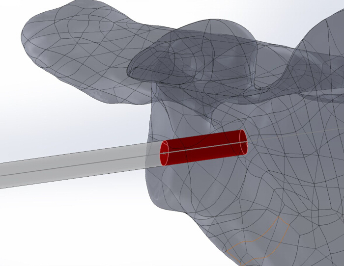
Figure 1: Three-dimensional reconstructed scapular model with a simulated central peg. A cylindrical 7.5 mm-diameter central peg is shown within the reconstructed scapula. The red segment represents the portion of the peg contained within the scapular bone; the gray segment shows the peg axis outside the entry surface. Please click here to view a larger version of this figure.

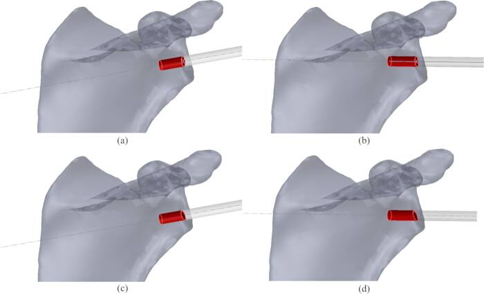
Figure 2: Four simulated central peg placement strategies. (A) Method a: Glenoid-center entry along the standard centerline (SCL). (B) Method b: Glenoid-center entry along the alternative centerline (ACL). (C) Method c: Entry 12 mm superior to the inferior glenoid rim along a trajectory parallel to the SCL. (D) Method d: Entry 12 mm superior to the inferior glenoid rim along a trajectory parallel to the ACL. The red cylinder represents the 7.5 mm-diameter central peg, and the gray extension indicates its trajectory. Please click here to view a larger version of this figure.

4. Measurement of maximum contained peg depth and cortical penetration

For each scapular model and placement method, an assembly constraint was used to place the center of the peg end face at the selected entry point. The peg axis was aligned with the SCL, ACL, or the corresponding parallel trajectory.

The entry point and trajectory were confirmed in the lateral en face, axial, and superior or inferior views. A section view was used when necessary to inspect the peg within the scapular vault. The peg was translated medially along its axis while the entry-point and trajectory constraints were maintained. Interference analysis was used to inspect the peg–bone relationship after each adjustment. Translation was stopped at the greatest depth at which the complete cylindrical peg remained within or tangent to the external cortical boundary and no portion projected beyond the cortex.

The distance from the glenoid entry point to the limiting distal end of the peg was recorded as the maximum contained peg depth in millimeters. The value was recorded before the assembly configuration was changed. The assembly was repeated with nominal peg lengths of 15, 20, and 25 mm. A configuration was classified as contained when the entire peg was inside or tangent to the cortical boundary and as cortical penetration when any part of the peg extended beyond the external cortex.

5. Angular-deviation simulations

The entry point, initial trajectory, and local coordinate system established for the selected method were retained (Figure 3). The scapula was displayed from the lateral side of the glenoid while viewed medially along the +z trajectory, and the same working view was used for Figure 3 and Figure 4.

With the entry point fixed, a deviated reference trajectory was created at a polar angle α of 5° from the initial +z trajectory. The construction was repeated for α = 10° and 15°. The entry point remained unchanged when the polar angle was altered. The azimuth θ was defined in the local x–y plane and increased clockwise in the lateral-to-medial working view. The directional convention was defined as θ = 0° superiorly (+y), 90° posteriorly (+x), 180° inferiorly (−y), and 270° anteriorly (−x).

For each polar angle α, the deviation direction was rotated clockwise about the initial +z trajectory from θ = 0° to 345° in 15° increments, generating 24 azimuthal directions. The viewing direction remained lateral-to-medial throughout the rotation. At every α–θ combination, the 7.5 mm peg was aligned with the deviated trajectory, and the maximum contained peg depth was determined using the procedure described above. The 24-direction sequence was repeated for all three polar deviations, all four placement methods, and all 100 scapular models. The same clockwise azimuth convention was applied to the directional results and Figure 4.

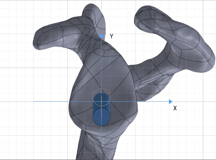
Figure 3: Local coordinate system and working view for angular-deviation analysis. The scapula is displayed from the lateral side of the glenoid while looking medially along the initial +z peg trajectory. In the plane parallel to the glenoid surface, +x points posteriorly and +y superiorly; −x and −y indicate anterior and inferior. Azimuth increases clockwise in this lateral-to-medial view: 0° is superior (+y), 90° posterior (+x), 180° inferior (−y), and 270° anterior (−x). Figures 3 and 4 use the same viewing direction and azimuth convention. Please click here to view a larger version of this figure.

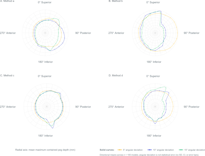
Figure 4: Directional maximum contained peg depth under simulated angular deviations. Panels A–D correspond to methods a–d. The plots use the same lateral-to-medial view as Figure 3, and azimuth increases clockwise from 0° superior through 90° posterior, 180° inferior, and 270° anterior in 15° increments. The radial axis is the mean maximum contained peg depth (mm) across 100 models. Solid yellow, blue, and green curves denote imposed polar deviations of 5°, 10°, and 15°, respectively; deviation describes trajectory offset and is not a statistical error estimate. Points are directional means. No SD, confidence interval, or error bars are displayed. Please click here to view a larger version of this figure.

6. Repeated measurements and resolution of disagreements

Two observers independently repeated all continuous depth measurements in two sessions. The final continuous value for each model and configuration was the mean of the four accepted readings (two observers × two sessions). If the review identified an incorrect landmark, trajectory, or cortical boundary, a senior radiologist confirmed the anatomical setup, and the affected observer repeated the measurement. The corrected reading replaced the invalid reading before calculation of the four-reading mean. The senior radiologist did not supply a fifth depth value.

Each observer/session also classified cortical penetration for each nominal peg length. When the four binary classifications were discordant, the senior radiologist re-examined the 3D model and assigned the final binary status used in the analysis. Inter-rater reliability for continuous depth was evaluated from each observer’s two-session mean using a two-way random-effects, absolute-agreement intraclass correlation coefficient (ICC). Intra-rater reliability was evaluated by comparing sessions using a two-way mixed-effects, absolute-agreement ICC.

Figure 5 summarizes patient selection, CT acquisition, 3D reconstruction, coordinate definition, the four placement strategies, nominal peg-length simulation, angular-deviation testing, outcome determination, and paired statistical analysis.

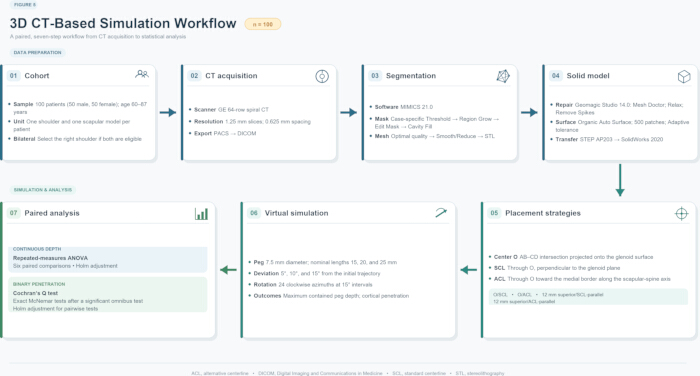
Figure 5: Overall 3D CT-based simulation workflow. The schematic summarizes selection of 100 unique patients (one shoulder and one scapular model per patient), CT acquisition, DICOM-based 3D reconstruction, coordinate and strategy definition, simulation of 15, 20, and 25 mm peg lengths, 5°, 10°, and 15° angular deviations at 15° azimuthal intervals, determination of maximum contained peg depth and adjudicated cortical penetration, and paired statistical analysis. Please click here to view a larger version of this figure.

7. Data analysis

For each nominal peg length and placement method, the adjudicated cortical-penetration outcome was summarized as n (%). Maximum contained peg depth was summarized as mean ± standard deviation (SD) and range. For angular-deviation analyses, the mean maximum contained peg depth across the 24 azimuths was calculated for each method and polar deviation, and these directional means were used to construct polar plots.

Data were managed, and descriptive summaries were calculated using spreadsheet software. Inferential analyses were performed using statistical analysis software. Because all four placement methods were evaluated in every scapular model, initial maximum contained peg depths were compared using one-factor repeated-measures analysis of variance (ANOVA). After a significant omnibus result, paired post hoc comparisons were conducted, and the family-wise error rate across the six method pairs was controlled with the Holm procedure. At each nominal peg length, the four paired binary penetration outcomes were compared using Cochran’s Q test. Pairwise exact McNemar tests with Holm adjustment were performed only if the omnibus test was significant. Two-sided tests were used with α = 0.05.

Результаты

Comparison of four placement approaches

The four placement strategies differed in initial maximum contained peg depth (Table 1). Method b achieved the greatest mean depth (24.99 ± 3.64 mm), whereas method a showed the greatest variability (SD, 4.07 mm). The observed ranges were 13–34 mm, 11–32 mm, 11–28 mm, and 13–27 mm for methods a–d, respectively. Repeated-measures ANOVA showed an overall difference (F(3,297) = 33.00, P = 1.95 × 10⁻¹⁸). Holm-adjusted paired comparisons were significant for a versus b (adjusted P = 0.00145), a versus c (adjusted P = 0.000159), a versus d (adjusted P = 2.61 × 10⁻⁶), b versus c (adjusted P = 4.28 × 10⁻¹¹), and b versus d (adjusted P = 2.27 × 10⁻¹²). The c-versus-d comparison was not significant (adjusted P = 0.0924).

Simulated cortical penetration increased numerically with peg length (Table 2). At 15 mm, penetration occurred in 4/100 (4%), 3/100 (3%), 3/100 (3%), and 5/100 (5%) models for methods a–d, respectively; the paired comparison among methods was not significant (Cochran’s Q(3) = 0.77, P = 0.857). At 20 mm, the corresponding frequencies were 13/100 (13%), 11/100 (11%), 10/100 (10%), and 14/100 (14%) (Q(3) = 1.13, P = 0.769). At 25 mm, method b had the numerically lowest frequency, 46/100 (46%), compared with 52/100 (52%), 56/100 (56%), and 61/100 (61%) for methods a, c, and d; however, the overall paired comparison remained nonsignificant (Q(3) = 6.44, P = 0.092). Because no Cochran’s Q test was significant, pairwise McNemar tests were not interpreted.

Effect of angular deviation on placement depth

Mean and summed maximum contained peg depths were calculated across the 24 sampled azimuths for each placement method and angular deviation (Figure 4; Table 3). At 5°, method b had the greatest mean depth (24.91 mm; summed depth, 597.76 mm). At 10° and 15°, method c had the greatest mean depths (20.23 and 18.29 mm; summed depths, 485.59 and 438.92 mm, respectively). Mean depth decreased from 5° – 15° for methods a, b, and d; method c increased slightly from 5° – 10° before decreasing at 15°.

For method a, maximum directional depths occurred at 0°, 15°, and 30° for deviations of 5°, 10°, and 15°, respectively, with corresponding maxima of 23.72, 20.39, and 18.84 mm. Minimum depths occurred at 180°, 195°, and 210°, respectively (Figure 4A). For method b, maximum directional depths occurred at 30°, 45°, and 60° for deviations of 5°, 10°, and 15°, respectively, with corresponding maxima of 25.89, 17.87, and 14.45 mm. The corresponding minima occurred at 210°, 225°, and 240° (Figure 4B). For method c, maximum directional depths occurred at 75°, 75°, and 90° for deviations of 5°, 10°, and 15°, respectively, with corresponding maxima of 20.94, 21.54, and 19.68 mm. The corresponding minima occurred at 255°, 255°, and 270° (Figure 4C). For method d, maximum directional depths occurred at 105°, 120°, and 120° for deviations of 5°, 10°, and 15°, respectively, with corresponding maxima of 19.04, 18.60, and 18.23 mm. The corresponding minima occurred at 285°, 300°, and 300° (Figure 4D).

Inter-rater and intra-rater agreement were excellent. For the four initial-placement methods, inter-rater single-measure ICC values ranged from 0.979 – 0.993, and average-measure ICC values ranged from 0.990 – 0.996. The corresponding intra-rater ranges were 0.993–0.997 and 0.996–0.999, respectively. Across the directional-deviation datasets, inter-rater single- and average-measure ICC values ranged from 0.984 – 0.997 and from 0.992 – 0.998, respectively; the corresponding intra-rater ranges were 0.990–0.998 and 0.995–0.999.

Placement method	Mean ± SD (mm)	Maximum (mm)	Minimum (mm)
a	23.94 ± 4.07	34	13
b	24.99 ± 3.64	32	11
c	22.31 ± 2.44	28	11
d	21.69 ± 2.73	27	13
Maximum contained peg depth for the four simulated central peg placement methods Values are based on 100 paired scapular models (one model per patient) and are reported in millimeters as mean ± SD and range. Method a: glenoid-center entry along the standard centerline (SCL); method b: glenoid-center entry along the alternative centerline (ACL); method c: entry 12 mm superior to the inferior glenoid rim along a trajectory parallel to the SCL; method d: the same superior entry along a trajectory parallel to the ACL. Repeated-measures ANOVA: F(3,297) = 33.00, P = 1.95 × 10⁻¹⁸. Holm-adjusted paired comparisons were significant for all pairs except c versus d (adjusted P = 0.0924).

Table 1: Maximum contained peg depth for four simulated placement methods. Values are based on 100 scapular models (one model per patient) and are reported in millimeters as mean ± SD and range. Method a: glenoid-center entry along the SCL; method b: glenoid-center entry along the ACL; method c: entry 12 mm superior to the inferior glenoid rim along a trajectory parallel to the SCL; method d: the same superior entry along a trajectory parallel to the ACL. Repeated-measures ANOVA: F(3,297) = 33.00, P = 1.95 × 10⁻¹⁸. Holm-adjusted paired comparisons were significant for all pairs except c versus d (adjusted P = 0.0924).

Method	15 mm peg: Penetration, n (%)	15 mm peg: Contained, n (%)	20 mm peg: Penetration, n (%)	20 mm peg: Contained, n (%)	25 mm peg: Penetration, n (%)	25 mm peg: Contained, n (%)
a	4 (4%)	96 (96%)	13 (13%)	87 (87%)	52 (52%)	48 (48%)
b	3 (3%)	97 (97%)	11 (11%)	89 (89%)	46 (46%)	54 (54%)
c	3 (3%)	97 (97%)	10 (10%)	90 (90%)	56 (56%)	44 (44%)
d	5 (5%)	95 (95%)	14 (14%)	86 (86%)	61 (61%)	39 (39%)
Results are adjudicated binary outcomes reported as n (%), with 100 paired scapular models per method and peg length. Cochran’s Q tests comparing the four methods were nonsignificant at 15 mm (Q(3) = 0.77, P = 0.857), 20 mm (Q(3) = 1.13, P = 0.769), and 25 mm (Q(3) = 6.44, P = 0.092). Method a: glenoid-center entry along the standard centerline (SCL). Method b: glenoid-center entry along the alternative centerline (ACL). Method c: entry 12 mm superior to the inferior glenoid rim along a trajectory parallel to the SCL. Method d: the same superior entry along a trajectory parallel to the ACL.

Table 2: Simulated cortical penetration and containment by nominal peg length and placement method. Results are adjudicated binary outcomes reported as n (%), with 100 paired scapular models per method and peg length. Method a: glenoid-center entry along the SCL; method b: glenoid-center entry along the ACL; method c: entry 12 mm superior to the inferior glenoid rim along a trajectory parallel to the SCL; method d: the same superior entry along a trajectory parallel to the ACL. Cochran’s Q tests comparing the four methods were nonsignificant at 15 mm (P = 0.857), 20 mm (P = 0.769), and 25 mm (P = 0.092).

Placement method	Angular deviation	Contained depth (mm)
		Mean	Sum
a	5°	22.97	551.36
	10°	19.56	469.51
	15°	17.94	430.44
b	5°	24.91	597.76
	10°	16.81	403.32
	15°	13.3	319.19
c	5°	19.72	473.3
	10°	20.23	485.59
	15°	18.29	438.92
d	5°	17.57	421.75
	10°	17.06	409.38
	15°	16.61	398.59
Maximum contained peg depth under simulated angular deviations. Depth is reported in millimeters. At each azimuth, depth was averaged across the 100 models; the reported mean is the average of the 24 directional means sampled every 15°, and the sum is their total. In the lateral-to-medial working view, azimuth increases clockwise from 0° superior through 90° posterior, 180° inferior, and 270° anterior. Method a: glenoid-center/SCL; method b: glenoid-center/ACL; method c: 12 mm superior/SCL-parallel; method d: 12 mm superior/ACL-parallel.

Table 3: Maximum contained peg depth under simulated angular deviations. Depth is reported in millimeters. At each azimuth, depth was averaged across the 100 models; the reported mean is the average of the 24 directional means sampled every 15°, and the sum is their total. In the lateral-to-medial working view, azimuth increases clockwise from 0° superior through 90° posterior, 180° inferior, and 270° anterior. Methods a–d is defined as in Table 1.

DATA AVAILABILITY:

The de-identified observer- and session-level maximum-contained-peg-depth measurements, model-level penetration status by peg length, and observer- and session-level directional-depth measurements supporting this study are publicly available in Zenodo at https://doi.org/10.5281/zenodo.22699931.

Обсуждение

This study used CT-based 3D modeling to compare simulated cortical penetration and maximum contained peg depth for four central peg placement strategies. Similar CT-based anatomical simulation has been used to reconstruct glenoid bone stock and evaluate a virtual central peg¹³. Preoperative planning, navigation, and patient-specific instrumentation may improve component-positioning accuracy^{14,15,16,17,18,19}, but the present work did not test an operative technique. Its results should therefore be interpreted as geometric simulation data rather than evidence of clinical safety or validated intraoperative performance.

Two entry points, the glenoid center and a point 12 mm superior to the inferior rim, were evaluated with the SCL and ACL. A central peg diameter of 7.5 mm represented a commonly used clinical design²⁰. Matsuki et al.²¹ reported 3D glenoid dimensions and orientation, and Jeong et al.¹³ incorporated central peg geometry into an anatomical simulation of glenoid bone stock. In the present dataset, method b provided the greatest initial mean maximum contained peg depth and the numerically lowest 25 mm penetration frequency, although the paired penetration comparison was not significant. At 10° and 15° deviations, the 12 mm superior entry point preserved greater mean depth than the corresponding glenoid-center method for both trajectories; at 5°, the glenoid-center methods retained greater depth. Thus, the effect of the entry point depended on both the magnitude of the deviation and the trajectory.

Trajectory orientation also affected maximum contained peg depth. Frankle et al.⁹ reported maximum insertion distances of 28.6 ± 4.1 mm for the SCL and 42.7 ± 19.1 mm for the ACL in normal glenoids, values greater than those in the present study. This difference may reflect the present simulation’s use of the full 7.5 mm peg volume and an explicit cortical-containment endpoint. In the directional simulations, the ACL-based glenoid-center method showed a marked reduction in mean depth as deviation increased (24.91, 16.81, and 13.30 mm at 5°, 10°, and 15°), whereas the corresponding SCL method decreased from 22.97 – 19.56 and 17.94 mm.

The directional simulations showed method-specific shifts in the direction of maximum depth as deviation increased. The maxima shifted from 0° – 15° – 30° for method a and from 30° – 45° – 60° for method b. Method c showed maxima at 75°, 75°, and 90°, whereas method d showed maxima at 105°, 120°, and 120°. The corresponding minimum directions were approximately opposite the maxima. These patterns describe the geometry of the simulated models and require experimental validation before clinical interpretation.

This study has several limitations. First, the cohort was deliberately restricted to those with relatively preserved glenoid anatomy and was excluded from those with radiographically evident osteoarthritis or rheumatoid arthritis. It therefore does not represent many RTSA candidates with erosion, deformity, or bone deficiency, and the ranking of strategies may differ in pathological glenoids. Second, measurements were made in a controlled virtual environment. Although inter-rater and intra-rater reliability were excellent, intraoperative landmark reproducibility and placement accuracy were not tested. Third, only a 7.5 mm straight central peg was modeled. Coatings, materials, threads, curvature, baseplate diameter, and other design features may alter the bone–implant interface; stress, strain, micromotion, and fixation strength were not assessed. Alternative approaches to studying these placement strategies include cadaveric validation, navigation-based implantation studies, and biomechanical testing, which could evaluate aspects of implantation accuracy and fixation that cannot be assessed in a CT-based geometric simulation. Future studies should extend this work to pathological glenoid cohorts and multiple implant designs, and include cadaveric or clinical validation to assess the applicability of the simulated findings.

In conclusion, this 3D CT-based simulation identified method-specific differences in maximum contained peg depth. Method b provided the greatest initial mean depth and the numerically lowest 25 mm cortical-penetration frequency, but the paired penetration comparison was not statistically significant. Under angular deviation, method b retained the greatest mean depth at 5°, whereas method c retained the greatest mean depth at 10° and 15°. These geometric findings require experimental or clinical validation before operative use.

Материалы

Список материалов, использованных в этой статье

Имя	Компания	Каталожный номер	Комментарии
64-slice spiral CT scanner	General Electric Company, USA	N/A	Used for preoperative CT image acquisition
Geomagic Studio software	3D Systems, Rock Hill, SC, USA	Version 14	Used for model surface processing and smoothing
Mimics software	Materialise, Leuven, Belgium	Version 21	Used for 3D reconstruction of scapular models from CT images
Shoulder CT dataset	Hospital database	N/A	Used for preoperative CT image acquisition
SolidWorks software	Dassault Systèmes, Vélizy-Villacoublay, France	Version 2020	Used for virtual implantation design and measurement