Near Real-Time Quantitative Ultrasound Imaging Using an Ultra-Portable Handheld Ultrasound System

Краткое содержание

This protocol demonstrates near real-time quantitative ultrasound imaging using an ultra-portable handheld ultrasound system to acquire radiofrequency data, estimate quantitative tissue parameters, and visualize parameter maps for point-of-care tissue characterization.

Аннотация

Clinical ultrasound is widely used because of its low cost, portability, safety, and real-time imaging capability, making it well suited for point-of-care applications. However, conventional B-mode imaging is inherently qualitative and primarily sensitive to tissue morphology. Quantitative ultrasound (QUS) methods exploit information contained in backscattered radiofrequency (RF) signals to extract fundamental acoustic tissue properties, such as the backscatter coefficient (BSC) and attenuation, which more directly quantify tissue microstructure and provide complementary information to B-mode imaging. Although QUS methods have been implemented on conventional cart-based ultrasound scanners, their integration into portable handheld systems remains limited. Motivated by the growing availability and clinical potential of ultra-portable ultrasound devices, this protocol presents a QUS imaging pipeline implemented on the DKPOC probe (portable linear ultrasound probe; Vermon SA, Tours, France), which interfaces directly with a laptop through a USB-C connection. The protocol integrates multiple QUS processing methods based on spectral analysis and envelope statistics of RF data acquired using focused-wave or plane-wave transmit modes. QUS processing begins with a user-defined region of interest (ROI). The reference phantom method is used to estimate the BSC and attenuation within sliding sub-ROIs. Model-based fitting of the estimated BSC is then performed to extract tissue microstructure-related parameters, including effective scatterer diameter and effective acoustic concentration. In addition, envelope statistics parameters are estimated using three probability density functions. Computed QUS parameter maps are displayed as translucent color overlays on corresponding B-mode images. The workflow is implemented in a numerical computing software–based graphical user interface, enabling near real-time QUS processing, parameter map visualization, interactive parameter adjustment, and rapid evaluation of different processing configurations. The pipeline is adaptable to different imaging sequences and ultrasound probes, providing a practical framework for quantitative point-of-care ultrasound imaging and clinician-led QUS studies in human subjects.

Введение

Clinical ultrasound imaging is widely used in medical practice because of its low cost, portability, safety, and ability to provide real-time visualization. These attributes make this modality well suited for point-of-care applications, where rapid bedside assessment is essential for clinical decision-making. Despite these advantages, conventional ultrasound imaging is predominantly based on B-mode imaging, which is inherently qualitative and provides information primarily related to tissue morphology through differences in acoustic impedance at tissue boundaries. This limits its ability to characterize subtle changes in tissue microstructure that may carry clinically significant diagnostic information. Consequently, because of the lack of quantitative information, diagnosis and prognosis are often subjective and prone to interobserver and intraobserver variability^1,2,3.

Quantitative ultrasound (QUS) methods, in contrast, exploit information contained in backscattered radiofrequency (RF) signals rather than relying solely on echo amplitudes. QUS methods extract fundamental acoustic tissue properties, including the backscatter coefficient (BSC) and attenuation, which more directly reflect tissue microstructure and provide quantitative information complementary to conventional B-mode imaging. Scattering model-based fitting of the estimated BSC further yields quantitative parameters that relate more directly to tissue microstructural properties^4,5,6. Fitting a Gaussian scattering model to the estimated BSC yields two QUS parameters: the effective scatterer diameter (ESD) and the effective acoustic concentration (EAC)⁵. Similarly, fitting a linear model to the estimated BSC yields three QUS parameters: spectral slope (SS), spectral intercept (I0), and mid-band fit (MBF)⁶. Because these QUS parameters are derived from fundamental acoustic tissue properties, they are independent of imaging system settings and operator interpretation, providing more objective quantitative tissue descriptors. Their quantitative nature also enables disease follow-up and treatment response monitoring. QUS parameters have demonstrated diagnostic utility across a range of applications, including prediction of breast cancer treatment response⁷, identification of cancerous regions in the prostate⁸ and thyroid⁹, and classification of metastatic lymph nodes^10,11,12. Similarly, attenuation-based QUS parameters have shown promise for tissue characterization, including differentiation of normal and steatotic liver tissue^13,14 and detection of malignant and benign tumors¹⁵. In addition to spectral-based methods, envelope statistics-based approaches provide another class of QUS parameters obtained by fitting envelope-detected RF echo values to theoretical probability density functions, such as the Rayleigh, Nakagami¹⁶, and Homodyned-K (H-K)¹⁷ distributions. Envelope statistics-based QUS parameters are particularly sensitive to scatterer number density and spatial organization and have similarly demonstrated utility for tissue characterization in applications including breast mass classification¹⁸ and hepatic steatosis assessment¹⁹. These relationships arise because the interaction of ultrasound waves with tissue depends on several factors, including the size, concentration, spatial arrangement, and acoustic impedance contrast of tissue microstructures relative to the imaging wavelength. Changes in tissue composition or organization alter the frequency content, amplitude distribution, and spatial statistics of the backscattered RF signal, which can be quantified using QUS parameters.

Over the past decade, QUS methods have been extensively developed and validated using conventional cart-based ultrasound systems^20,21. However, these systems are large and typically confined to clinical or laboratory settings, limiting the broader accessibility of QUS imaging. In recent years, ultra-portable handheld ultrasound devices that connect directly to smartphones or laptops have become increasingly available, offering a compelling opportunity to extend ultrasound imaging to point-of-care settings^22,23. However, the integration of QUS methods into ultra-portable handheld ultrasound devices remains limited, largely because of restricted access to RF data and the computational demands of QUS processing on compact hardware. While some efforts have been made to implement QUS methods on portable platforms²⁴, a comprehensive, user-friendly pipeline integrating spectral-based and envelope statistics-based QUS processing with near real-time visualization has not yet been demonstrated on an ultra-portable system. Motivated by the increasing availability and clinical potential of ultra-portable ultrasound systems with access to RF data, we present a QUS imaging pipeline with a MATLAB (numerical computing software)-based graphical user interface (GUI), implemented using the portable linear ultrasound probe, interfaced with a laptop through a USB-C connection. The primary contribution of this work is the system integration and software implementation of multiple spectral and envelope statistics-based QUS methods into a unified software pipeline for the ultra-portable ultrasound platform. By leveraging access to beamformed RF data, the proposed implementation enables interactive near real-time QUS processing, visualization, and parameter tuning, making multiparametric QUS imaging readily accessible for point-of-care applications using the portable ultrasound platform.

This compact, ultra-portable system eliminates the need for bulky cart-based hardware while retaining the ability to acquire RF data using user-defined transmit and receive aperture configurations. The system provides FPGA-based real-time beamforming for focused-wave (FW) and plane-wave (PW) linear scan acquisitions, two commonly used transmit configurations in clinical ultrasound imaging, while also allowing access to channel data for custom acquisition and beamforming strategies. The developed pipeline integrates multiple QUS processing methods based on spectral analysis and envelope statistics of beamformed RF data acquired using both focused-wave and plane-wave transmit configurations. Spectral-based QUS processing is performed using the reference phantom method²⁵ to estimate the BSC and attenuation within sliding sub-regions of interest (sub-ROIs) defined inside a user-defined ROI, from which model-based fitting is used to extract QUS parameters related to tissue microstructure. Envelope statistics parameters are estimated from the envelope amplitudes within each sub-ROI using multiple probability distribution models. The computed QUS parameter maps are visualized as translucent color overlays on corresponding B-mode images, enabling near real-time spatial assessment of tissue acoustic properties. The goal of the present protocol is to demonstrate a near real-time QUS imaging pipeline that simplifies QUS imaging and brings it closer to the clinical environment. This protocol is intended for researchers and clinicians interested in quantitative point-of-care ultrasound applications, providing a flexible framework for translational biomedical ultrasound research and clinician-led QUS studies in human subjects. The following protocol describes system setup, RF data acquisition, QUS processing, and parameter visualization using the developed numerical computing software–based GUI on the portable ultrasound platform.

Протокол

No human participants or live animals were involved. Therefore, institutional human research ethics approval and animal care and use committee approval were not required.

1. System Setup and GUI Initialization

1. Connect the linear ultrasound probe to the laptop using the USB-C cable, as shown in Figure 1. Ensure that the USB-C port is compatible with Thunderbolt technology (high-speed hardware interface) to support the high-speed data transfer required for real-time RF data streaming.
2. Press the power button on the probe, as annotated in Figure 1. Confirm that the red light-emitting diode (LED) indicator is illuminated, indicating that the probe is powered and ready for use.
3. Launch the numerical computing software (version 2018a or later) and navigate to the directory containing the GUI script. Open the script named GUI_v1_main1.m.
4. Before running the GUI, install the numerical computing software R2018a or later (R2025b recommended) together with the required toolboxes: Signal Processing Toolbox, Statistics and Machine Learning Toolbox (statistical analysis software toolbox), and Curve Fitting Toolbox.
   1. Install the device acquisition software (version 2.1.0) and the associated device drivers and MEX functions for data acquisition provided by the manufacturer.
   2. Add the folders containing the GUI and QUS processing code to the numerical computing software search path. Verify that the ultrasound probe is recognized by the operating system before launching the GUI.
5. Run the script to initialize the portable ultrasound system. Upon successful initialization, verify that the main GUI window opens, as shown in Figure 2. Monitor the numerical computing software Command Window and confirm that the message “Probe state::READY” is displayed before proceeding. Note that initialization may take several seconds while the system establishes communication with the probe.
6. If the message “Probe state::READY” is not displayed, verify that the ultrasound probe is connected, powered, and recognized by the operating system. Verify that the device acquisition software (version 2.1.0), the associated device drivers, and MEX functions are correctly installed.
   1. Restart the GUI and repeat the initialization. Proceed only after the message “Probe state::READY” appears in the numerical computing software Command Window.
   2. Refer to the device manual supplied by the manufacturer for additional troubleshooting guidance.

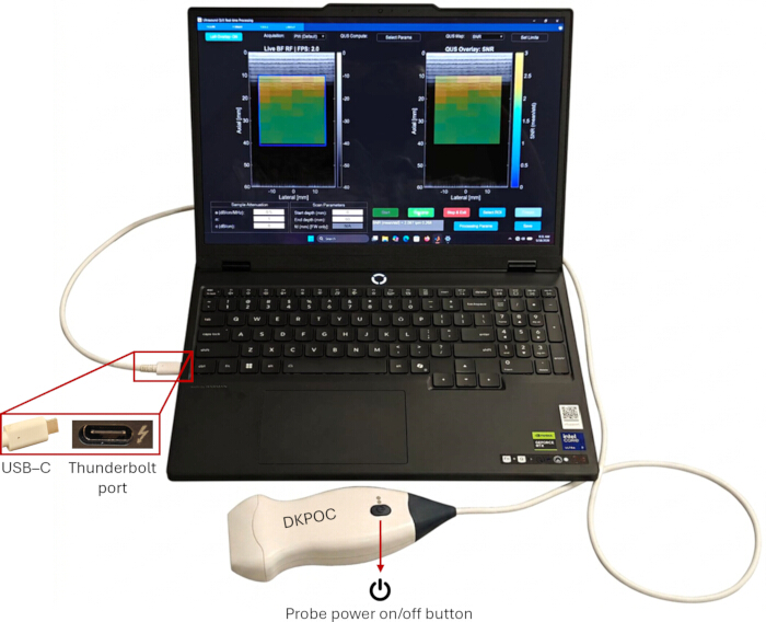
Figure 1. Experimental setup of the portable quantitative ultrasound (QUS) imaging system. A linear ultrasound probe is connected directly to a laptop using a USB-C cable through a high-speed hardware interface for real-time radiofrequency (RF) data transfer. The location of the probe power button is indicated. Please click here to view a larger version of this figure.

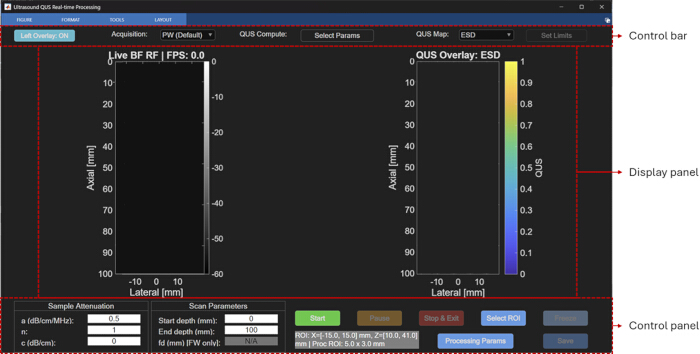
Figure 2. Main graphical user interface (GUI) of the portable quantitative ultrasound (QUS) imaging software. The GUI consists of a control bar, display panel, and control panel. The display panel contains the live B-mode image and the quantitative ultrasound parameter overlay window used for near real-time visualization. Please click here to view a larger version of this figure.

2. GUI Overview and Default Settings

1. Verify that the GUI titled “Ultrasound QUS Processing” has loaded successfully. Confirm that the GUI consists of three main components, as annotated in Figure 2: a top control bar, a bottom control panel, and a central display panel containing two image windows. Verify that the left window, titled “Live BF RF | FPS: 0.0,” displays the live B-mode image and that the right window, titled “QUS Overlay: ESD,” displays the QUS parameter map overlaid on the B-mode image. Note that both windows remain blank until data acquisition is started.
2. Review the controls located in the top control bar.
   1. Verify that the “Left Overlay: ON” toggle button controls whether the QUS parameter map overlay is displayed on the left live B-mode image. Note that the QUS overlay in the right image window always remains enabled. Use this toggle when comparing QUS parameters across different regions.
   2. Verify that the “Acquisition” drop-down menu (Figure 3A) is set to “PW (Default),” corresponding to plane-wave transmit mode.
   3. Verify that the “Select Params” button (Figure 3B) opens the parameter selection window described in Step 2.3.
   4. Verify that the “QUS Map” drop-down menu (Figure 3C) is set to “ESD” by default. This setting determines the QUS parameter displayed as the color overlay in the right display window.
   5. Verify that the “Set Limits” button (Figure 3D), which adjusts the color scale limits of the QUS parameter map, is inactive before data acquisition begins.
3. Click “Select Params” to open the parameter selection window, as shown in Figure 3B. Verify that the following parameters are selected by default for near real-time processing.
   1. Gaussian scattering model fit to the BSC: ESD and EAC.
   2. Linear model fit to the BSC: MBF, SS, and I0.
   3. Envelope statistics-based Nakagami parameters: Nakagami scale parameter and Nakagami shape parameter.
   4. Add additional parameters, including Rayleigh signal-to-noise ratio (SNR), H-K parameters, and attenuation-based parameters (attenuation coefficient and attenuation intercept), by holding Shift while selecting the desired parameters. Click “Select All” to select all available parameters. Note that selecting a larger number of parameters reduces the processing frame rate, as discussed in the Representative Results and Discussion sections.
   5. Use the “Select ROI” button (Figure 3E) to activate the crosshair tool for selecting two diagonally opposite corners of a rectangular ROI on the B-mode image. Note that this function becomes available only after data acquisition has started.
      NOTE: The GUI automatically restores the default parameter configuration each time it is launched.
4. Review the two sections of the control panel.
   1. Verify that the “Sample Attenuation” section (Figure 3F) contains editable fields for the attenuation coefficient (a, dB/cm/MHz), exponent (n), and attenuation intercept (c, dB/cm), with default values of 0.5, 1, and 0, respectively. Use these values to compensate for two-way attenuation during QUS processing, as described in Steps 3.5–3.7.
   2. Verify that the “Scan Parameters” section (Figure 3G) contains editable fields for “Start depth (mm)” and “End depth (mm),” with default values of 0 mm and 100 mm, respectively. Verify that the “fd (mm) [FW only]” field specifies the transmit focal depth for focused-wave acquisition. Confirm that this field is inactive and displays “N/A” during plane-wave acquisition.
   3. Enter finite numeric values in the attenuation fields. Enter numeric scan depths, with the start depth ≥ 0 mm and the end depth greater than the start depth. If an invalid value is entered, acknowledge the warning; the field will revert to the current configuration value. In focused-wave mode, enter a numeric focal depth; the value is automatically rounded to the nearest 5 mm within the range of 10–75 mm.
5. Verify that the default ROI displayed at the bottom of the GUI is “ROI: X = [−15, 15] mm, Z = [10, 41] mm,” with a processing sub-ROI size of 5 mm × 3 mm. These values define the processing region and the dimensions of the sliding sub-ROI windows used for spectral analysis. Modify these values using the “Processing Params” button, as described in Step 2.6.
   ​NOTE: The default ROI and sub-ROI dimensions are predefined and remain fixed across all acquisition configurations. The ROI may be modified interactively during a paused acquisition using the “Select ROI” function.
6. Click “Processing Params” to open the processing parameters window, as shown in Figure 3H.
   1. Verify that “Axial ROI (mm)” defines the axial dimension of the processing sub-ROI.
   2. Verify that “Lateral ROI (mm)” defines the lateral dimension of the processing sub-ROI.
   3. Verify that “BW min (MHz)” and “BW max (MHz)” define the processing bandwidth used for estimating and fitting the BSC and attenuation (when selected in “Select Params”). For the portable ultrasound probe, the default bandwidth is 3–6.5 MHz, corresponding to the −6 dB bandwidth of the reference phantom RF power spectrum.
      NOTE: Select the processing bandwidth within the common −6 dB bandwidth of the sample and reference RF power spectra, excluding frequency regions with a low signal-to-noise ratio.

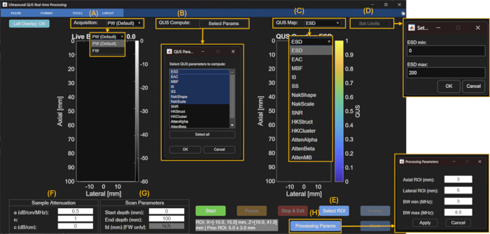
Figure 3. Annotated graphical user interface (GUI) controls used for quantitative ultrasound (QUS) acquisition and processing. (A) Acquisition mode selection. (B) QUS parameter selection window. (C) QUS parameter map selection menu. (D) Color scale adjustment window. (E) Region-of-interest (ROI) selection control. (F) Sample attenuation settings. (G) Scan parameter settings. (H) Processing parameter window for configuring sub-ROI dimensions and processing bandwidth. Please click here to view a larger version of this figure.

3. Scan Parameter Configuration and Data Acquisition

1. In the top control bar, select the desired transmit mode from the “Acquisition” drop-down menu. Select “PW” for plane-wave acquisition or “FW” for focused-wave acquisition.
2. In PW acquisition mode, generate quasi-plane-wave transmissions by applying transmit delays corresponding to a focal depth of approximately 1 m, providing a practical approximation of a plane-wave transmit field. In FW acquisition mode, apply transmit delays to focus the acoustic beam at a user-defined focal depth. In both acquisition modes, sequentially translate a moving 64-element transmit aperture across the probe aperture to generate 255 beamformed image lines.
   1. Select PW or FW from the “Acquisition” drop-down menu. The selected acquisition mode automatically configures the corresponding transmit delays, receive aperture configuration, and FPGA beamforming parameters. Acquire beamformed RF data using the ultrasound probe (6 MHz center frequency) at a sampling frequency of 24 MHz with a fixed 3-half-cycle (1.5-cycle) sinusoidal transmit pulse centered at the probe operating frequency.
3. If “FW” is selected, verify that the “fd (mm) [FW only]” field in the “Scan Parameters” section becomes active. Enter the desired focal depth in millimeters.
4. Select a focal depth between 10 mm and 75 mm in 5 mm increments. Use the default focal depth of 15 mm, unless a different focal depth is required. Position the focal depth near the center of the ROI to maximize lateral resolution. For example, when imaging a lymph node, position the focal depth near the center of the lymph node.
5. In the “Sample Attenuation” section of the control panel, verify or update the attenuation compensation parameters for the medium being imaged.
   1. Set the attenuation coefficient (a; dB/cm/MHz).
   2. Set the attenuation exponent (n).
   3. Set the attenuation intercept (c; dB/cm).
6. Use these parameters to compensate for frequency-dependent propagation losses during QUS processing according to Equation 1. The subscript ref denotes the reference phantom²⁶.
       (1)
   Here, , and f is the frequency (MHz).
7. Use the default sample values (α₀ = 0.5 dB/cm/MHz, n = 1, c = 0 dB/cm) for tissue-mimicking phantoms. Update these values to match the known or estimated attenuation properties of the medium when imaging other tissues, such as breast tissue^27,28.
   NOTE: Incorrect attenuation compensation values introduce bias into the estimated BSC. Attenuation compensation does not affect envelope statistics-based parameters because these parameters are estimated directly from the envelope amplitudes of the RF data.
   1. When the sample attenuation is unknown, select the attenuation-based linear fit parameters in the ‘QUS Compute: Select Parameters’ menu to obtain estimates of the attenuation coefficient and intercept maps²⁹. Enter the estimated attenuation coefficient and intercept corresponding to the depth of interest into the “Sample Attenuation” section for attenuation compensation during subsequent BSC estimation.
8. In the “Scan Parameters” section, set the “Start depth (mm)” and “End depth (mm)” fields to define the axial imaging range.
9. Use the default values of 0 and 100 mm, respectively, to image the full depth of the probe. Reduce the imaging depth to the ROI to improve the acquisition frame rate by reducing the amount of data acquired and processed per frame.
10. Click the green “Start” button to begin data acquisition.
    NOTE: Pressing “Start” initiates QUS processing automatically within the default ROI, and the selected parameter map is displayed as a color overlay on the corresponding B-mode image.
11. Verify that the left display window titled “Live BF RF” displays live B-mode images and that the current acquisition frame rate is shown as “FPS:” in the window title. Verify that the right display window titled “QUS Overlay: ESD” simultaneously displays the live B-mode image with a translucent color overlay of the selected QUS parameter from the “QUS Map” drop-down menu within the default ROI.
    1. Verify that the displayed B-mode image is free of visible motion artifacts and that adequate acoustic coupling has been maintained before proceeding with QUS processing. If significant probe or sample motion is observed, stabilize the probe and allow the QUS parameter maps to update before proceeding.
12. When a satisfactory B-mode image of the target tissue is displayed, click “Pause” to pause data acquisition.
13. Verify that the button label changes to “Resume,” allowing live acquisition to be restarted at any time.
14. Click “Select ROI” to define the ROI for QUS processing.
15. On the live B-mode image, select two diagonally opposite corners of the desired rectangular ROI. Verify that the selected ROI defines the spatial extent over which QUS processing will be performed using the sliding sub-regions of interest (sub-ROIs) specified in the “Processing Params” window (Step 2.6).
    1. Position the ROI over the tissue region of interest. If modifying the default sub-ROI dimensions, maintain the recommended minimum size of approximately 10 times the axial and lateral resolutions. For spectral-based QUS processing, position the ROI within the depth range for which reference phantom data are available (≤50 mm). For envelope statistics-based processing, position the ROI anywhere within the full imaging depth.
16. After defining the ROI, click “Resume” to restart live acquisition.
17. Verify that near real-time QUS processing and parameter map visualization begin automatically. Confirm that the right display window updates the displayed QUS parameter overlay according to the newly selected ROI.
    1. If parameter estimation fails because required inputs are blank, enter the missing inputs, and repeat the acquisition.
    2. As a quality check for spectral-based QUS parameter maps, verify that the BSC-based intercept (I0) and mid-band fit (MBF) maps do not exhibit a systematic depth-dependent gradient, which may indicate incorrect attenuation compensation.
    3. For Homodyned-K processing, identify saturated regions in the H-K Cluster map as failed parameter estimates; do not interpret these regions as valid QUS estimates.
18. To save the acquisition results, proceed to Step 5.
19. To terminate the session, click “Stop & Exit” to stop data acquisition and close the GUI.

4. QUS Processing and Visualization

1. Verify QUS Parameter Selection
   1. Click “Select Params” and verify that the desired QUS parameters are selected for computation, as described in Step 2.3.
   2. Verify that the “QUS Map” drop-down menu displays only the parameters selected in the “Select Params” window. 
2. Start QUS Processing
   1. After defining the ROI as described in Step 3.15, click “Resume” to restart data acquisition.
   2. Verify that near real-time QUS processing begins automatically. Confirm that all selected QUS parameters are computed simultaneously using the same sliding sub-ROIs defined in the “Processing Params” window (Step 2.6).
      NOTE: Successful computation is indicated by display of the selected QUS parameter map as a color overlay on the corresponding B-mode image. For failed parameter estimation and troubleshooting, refer to Step 3.17.1.
3. Spectral-Based Processing
   1. BSC Estimation: If BSC-based parameters are selected in “Select Params,” estimate the BSC within each sub-ROI using the reference phantom method (RPM)^25,26. The sample BSC for each sub-ROI is estimated using Equation 2 as follows:
        ​(2)
      Here, BSCref(f) is the frequency-dependent BSC of the reference phantom, NPS(f,z) is the normalized power spectrum, A(f,z) is the attenuation compensation term, T(f,z) accounts for transmission losses through the phantom membrane, f is frequency (MHz), and z is the axial distance from the probe surface to the midpoint of the current sub-ROI.
   2. Calculate the normalized power spectrum (NPS) for each sub-ROI using Equation 3.
         (3)
      Here, N is the number of RF segments within each sub-ROI;  is the power spectrum of the ith RF segment, calculated as the squared magnitude of its Fourier transform; and PS_ref is the average reference phantom power spectrum calculated using the same sub-ROI size and location.
      NOTE: The power spectrum (PS) is estimated as the mean squared magnitude of the FFT of all 3 mm axial RF segments within each 5 mm (lateral) × 3 mm (axial) sub-ROI using a rectangular window. An FFT length of 2048 points is used, with zero-padding applied as needed. For real-time processing, adjacent sub-ROIs are processed without overlap to maximize the frame rate.
   3. Gaussian Scattering Model: Fit the estimated BSC for each sub-ROI using the Gaussian scattering model (Equation 4):
         (4)
      Here, n is the scatterer number density, a_eff is the effective scatterer radius, γ₀ is the relative acoustic impedance mismatch, v_s is the sound speed, and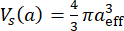  is the effective scatterer volume⁴.
   4. Estimate the ESD using Equation 5 as follows:
       (5)
   5. Estimate the EAC (dB/m³) using Equation 6 as follows:
        (6)
   6. Linear Spectral Parameters: Perform linear fitting of the estimated BSC to calculate the SS, I0, and MBF. Although these parameters do not directly represent scatterer size or concentration, they are sensitive to changes in tissue microstructure and are widely used for tissue characterization and classification studies³⁰.
   7. Attenuation Estimation: If attenuation-based parameters are selected in ‘Select Params,’ estimate the attenuation within each sub-ROI using the RPM²⁹. Estimate the sample attenuation using Equation 7:
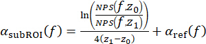         (7)
      Here, z₁ is the axial midpoint of the current sub-ROI, z₀ is the midpoint of the initial fixed reference sub-ROI, and  is the attenuation of the reference phantom.
      NOTE: This approach estimates the cumulative attenuation between the initial fixed sub-ROI and the current sub-ROI.
   8. Perform linear fitting of the estimated attenuation curve to calculate: attenuation coefficient, α₀ (AttenAlpha; dB/cm/MHz); attenuation intercept, c (AttenIntercept; dB/cm); and attenuation at the mid-band (AttenMB; dB/cm).
4. Reference Phantom
   1. Verify that the software automatically selects the appropriate reference phantom RF dataset according to the current acquisition settings.
   2. Use the pre-acquired reference phantom consisting of an agar-based material containing embedded 60 µm borosilicate glass beads and a 25 µm TPX (polymethylpentene) membrane.
   3. Calculate the reference phantom backscatter coefficient, , using Faran scattering theory³¹ and the following material properties: speed of sound (5640 m/s), density (2.5 g/cm³), and Poisson’s ratio (0.2).
   4. Use the reference phantom beamformed RF data supplied with the GUI for the PW and FW acquisition configurations supported by the GUI, including all available FW focal depths. The supplied reference dataset contains 20 frames for each configuration, acquired by slightly repositioning the probe between acquisitions to obtain independent speckle realizations. The corresponding .bin files provide the transmit, receive, and beamforming settings used for acquisition of the reference and sample RF data.
   5. To generate a new reference dataset (e.g., for recalibration), acquire beamformed RF data for each intended acquisition configuration by loading the corresponding .bin files into the Pulsarus software and following the RF acquisition procedure described in the ultrasound probe user manual.
   6. Use the characterized physical and acoustic properties of the reference phantom for BSC calculations.
      NOTE: The physical properties of the reference phantom, including the size and number density of the borosilicate glass beads, were provided by the phantom manufacturer. The acoustic properties of borosilicate glass used for BSC calculations were obtained from the experimental characterization reported by Millet J and Bourne N³². The attenuation properties of the reference phantom over the ultrasound probe processing bandwidth were experimentally estimated using the reference phantom method²⁶ with the well-characterized 18 µm phantom described by Rohrbach et al.⁸ as the attenuation reference.
   7. When generating a new reference phantom, use a uniform random distribution of glass bead scatterers at a sufficient number density (i.e., >10 scatterers per resolution cell) to produce fully developed speckle. Use a phantom with well-characterized frequency-dependent BSC and attenuation properties over the processing bandwidth.
5. Envelope Statistics Processing
   1. If envelope statistics parameters are selected in “Select Params,” estimate the envelope statistics parameters from the envelope amplitudes within each sub-ROI using the selected probability density function (PDF).
   2. Rayleigh SNR: Calculate the Rayleigh SNR as the ratio of the mean envelope intensity to the standard deviation of the envelope intensities within each sub-ROI.
   3. Interpret values approaching  as indicating a Rayleigh envelope distribution corresponding to fully developed speckle.
   4. Nakagami Distribution: Estimate the Nakagami distribution using Equation 8.
         (8)
      Here, Γ is the gamma function and U is the unit step function.
   5. Fit the Nakagami PDF using a maximum likelihood estimator to estimate shape parameter (m) and scale parameter (Ω).
      NOTE: Interpret: m < 1 as pre-Rayleigh scattering; m = 1 as Rayleigh scattering; and m > 1 as post-Rayleigh scattering.
   6. Estimate the Nakagami parameters using the numerical computing software’s fitdist() function (statistical analysis software toolbox) with the Nakagami distribution specified. The function estimates the Nakagami shape and scale parameters using the numerical computing software’s built-in maximum likelihood estimation procedure.
   7. H-K Distribution: Estimate the H-K distribution using Equation 9.
         (9)
      Here, J₀ is the zeroth-order Bessel function of the first kind; ε² and σ² represent the coherent and diffuse signal energies, respectively; and α is the scatterer clustering parameter.
   8. Estimate the H-K structure parameter (k) as the ratio of coherent to diffuse signal components (ε/σ).
   9. Estimate the H-K parameters using the first moment of intensity and two logarithmic moments³³.
   10. Use the XU estimator to estimate the Homodyned-K distribution parameters. The XU estimator was selected because it is a well-established and widely validated method for Homodyned-K parameter estimation in quantitative ultrasound studies^33,34. Although computationally intensive and therefore not suitable for near real-time implementation in the current pipeline, it provides a reliable reference implementation for demonstrating Homodyned-K parameter estimation. More computationally efficient Homodyned-K estimators have recently been reported^35,36 and will be evaluated for integration into future versions of the software to enable real-time processing.
   11. Identify unsuccessful Homodyned-K fits as saturated regions in the H-K Cluster map, as described in Step 3.17.3. Do not interpret these regions as valid QUS estimates.
   12. When higher frame rates are required, use Nakagami fitting and Rayleigh SNR estimation for near real-time processing. Use H-K fitting separately or during offline analysis because of its higher computational cost.
   13. Apply a base-10 logarithmic transformation to the dynamic range of Ω after estimating the Nakagami and H-K parameters to facilitate visualization across regions exhibiting large parameter variability.

5. Saving and Exporting QUS Results

1. Click “Pause” to pause live data acquisition.
2. Verify that the “Save” button becomes active. Note that the “Save” button remains inactive during live data acquisition.
3. Click “Save” to export the current acquisition data.
4. Verify that the software automatically creates a directory named “saved_data/YYYY-MM-DD/acqX”, where “YYYY-MM-DD” corresponds to the acquisition date and “acqX” corresponds to the acquisition number for that day.
   NOTE: The save directory is fixed to “saved_data” and cannot be configured through the GUI. If the destination acquisition folder already exists, an incremental suffix (e.g., acq_2, acq_3) is automatically appended to prevent overwriting. Each acquisition folder contains a screenshot of the GUI and a numerical computing software file (buffered_qus_capture.mat) containing the corresponding QUS parameter maps and buffered RF data from the previous 10 frames.
5. Verify that a .jpg image of the GUI has been exported to the acquisition directory.
6. Verify that a .mat file containing the exported QUS data structures has been exported to the acquisition directory.
7. Open the exported .mat file in the numerical computing software.
8. Verify that the param_struct data structure contains the processing parameters, including the sub-ROI dimensions, processing bandwidth, and assumed speed of sound.
9. Verify that the saveBuffer data structure contains the beamformed RF data corresponding to the current frame and the previous nine frames, together with the estimated QUS parameter maps and their spatial locations within the exported B-mode images.
   NOTE: The exported MAT-file contains a saveBuffer structure array representing the 10-frame acquisition buffer immediately preceding the save operation. Each element contains the computed QUS results (output), corresponding beamformed RF data (rf), lateral (x, mm) and axial (z, mm) coordinate vectors, and acquisition timestamp (timestamp). The MAT-file also contains a param_struct structure storing the processing parameters used for all buffered frames, including the ROI and sub-ROI definitions (roi, m), processing bandwidth (proc_bw, Hz), and speed of sound (c, m/s). Together, these data enable reproduction of QUS parameter estimation from the saved beamformed RF data, as described in Step 6.
   NOTE: Repeat the acquisition and saving procedure as needed for different imaging regions, acquisition settings, or processing configurations.

6. Offline Reprocessing and Visualization

1. Launch the numerical computing software and run the script “load_saved_data.m” to reload previously exported RF data and corresponding QUS parameter maps for offline visualization and reprocessing.
2. Select the desired buffered_qus_capture.mat file from the acquisition directory. Verify that the script loads the saved beamformed RF frames and corresponding QUS parameter maps into the offline visualization window, as shown in Figure 4.
   NOTE: No additional software, toolboxes, or external dependencies are required beyond those listed in Step 1.4. The load_saved_data.m script uses the exported MAT-file described in Step 5.9 for offline visualization and reprocessing.
3. Navigate through the saved image sequence using the scrollbar or the “Previous” and “Next” buttons.
4. Click “Processing Params” to modify the sub-ROI dimensions and processing bandwidth.
5. Click “Select ROI” to redefine the ROI.
6. Click “Recompute Frame” to recompute the QUS parameter maps for the current frame using the updated processing parameters and ROI.
   NOTE: Offline recomputation does not overwrite the original saved data. The original saveBuffer remains unchanged, and the recomputed QUS parameter maps are stored only in the numerical computing software workspace unless they are explicitly saved as a new dataset.
7. Click “Set Limits” to adjust the color scale of the displayed QUS parameter map during offline review.
8. Enter the desired minimum and maximum values for the selected parameter to update the displayed color scale.
   NOTE: Color scale adjustments apply only to the current offline visualization session and are not saved with the recomputed results. When the offline viewer is reopened, the default display limits are restored unless they are adjusted again.

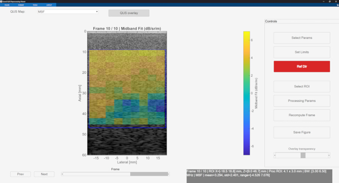
Figure 4. Offline quantitative ultrasound (QUS) visualization and reprocessing interface. Previously saved radiofrequency (RF) datasets are loaded using the load_saved_data.m script for offline visualization, frame navigation, region-of-interest (ROI) selection, parameter recomputation, and color scale adjustment. Please click here to view a larger version of this figure.

Результаты

BSC validation using tissue-mimicking phantoms

To validate the BSC-based QUS processing pipeline, BSC estimation was performed using an agar-based tissue-mimicking phantom containing 60 µm diameter borosilicate glass beads as the sample phantom and an agar-based phantom containing 18 µm diameter borosilicate glass beads as the reference phantom. These phantoms were selected because their scatterer size, material properties, and acoustic properties had been independently characterized, enabling comparison between experimentally estimated BSC values and theoretical BSC predictions. The structural and acoustic properties of both phantoms were known a priori. The attenuation properties of the 18 µm reference phantom consisted of an attenuation coefficient of 0.028 dB/cm/MHz^1.862 and exponent of 1.862, as reported in Rohrbach et. al.⁸. The 60 µm phantom had an attenuation coefficient of 0.34 dB/cm/MHz and an attenuation intercept of −0.8 dB/cm over the 3.5–6 MHz processing bandwidth.

BSC estimation was performed using the reference phantom method, as described in Step 4.3, for both PW and FW acquisition RF data with the focal depth fixed at 20 mm, as shown in Figure 5A–D. The theoretical BSC of the 60 µm phantom was computed using Faran scattering theory with the following borosilicate glass bead acoustic and mechanical properties: speed of sound of 5640 m/s, mass density of 2.5 g/cm³, and Poisson’s ratio of 0.2. Analysis was performed within a 30 mm × 15 mm ROI subdivided into 5 mm × 3 mm sliding sub-ROIs, as shown in Figure 5A–D. Figure 5E shows the estimated BSC curves for the 60 µm phantom averaged over the entire ROI using a single frame for both PW and FW acquisition modes, together with the theoretical BSC. At the mid-band frequency of 4.75 MHz, the estimated BSC using PW acquisition was −0.43 ± 1.60 dB/m/sr, whereas FW acquisition yielded a mean BSC of −0.80 ± 1.26 dB/m/sr. Figure 5F shows the estimated BSC curves averaged over 20 frames for both acquisition modes. Averaging over 20 frames reduced the variance of the estimated BSC curves and improved agreement with the theoretical BSC. At 4.75 MHz, the estimated mean BSC using PW acquisition increased to −0.25 ± 0.52 dB/m/sr, whereas FW acquisition yielded a mean BSC of −0.01 ± 0.51 dB/m/sr. The theoretical BSC at 4.75 MHz calculated using Faran scattering theory was -0.15 dB/m/sr. The close agreement between the estimated and theoretical BSC values at the mid-band frequency under both single-frame and 20-frame averaging conditions demonstrates that the pipeline generated BSC estimates consistent with the theoretical predictions.

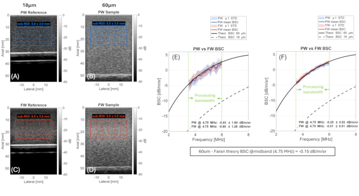
Figure 5. Validation of backscatter coefficient (BSC) estimation using tissue-mimicking phantoms with known scatterer sizes. (A–D) Plane-wave (PW) and focused-wave (FW) B-mode images of the reference and sample phantoms showing the processing region of interest (ROI) and sliding sub-regions of interest (sub-ROIs). (E,F) Estimated BSC curves obtained using single-frame averaging and 20-frame averaging compared with theoretical BSC values calculated using Faran scattering theory. Shaded regions represent ±1 standard deviation (SD). Please click here to view a larger version of this figure.

To further evaluate the BSC-based parameter estimation, Gaussian scattering model fitting and linear fitting were applied to the estimated BSC curves for both acquisition modes to obtain the ESD, EAC, SS, I0, and MBF. The estimated parameters, averaged over the entire ROI, are summarized in Table 1 for both single-frame and 20-frame averaging. The expected model parameters, obtained by applying the same fitting procedures to the theoretical Faran BSC curve, are presented in the final row of Table 1.

Acquisition	Number of frames	ESD (μm)	EAC (dB/m³)	SS  (dB/sr/m/MHz)	I0 (dB/sr/m)	MBF (dB/sr/m)
FW	1	74.6 ± 28.6	100 ± 7.20	2.83 ± 0.57	−14.0 ± 2.92	−0.49 ± 0.58
FW	20	84.3 ± 10.9	97.2 ± 3.07	2.68 ± 0.26	−13.1 ± 1.28	−0.3 ± 0.28
PW	1	77.6 ± 33.6	100 ± 13.1	2.74 ± 0.78	−13.9 ± 3.69	−0.86 ± 0.51
PW	20	85.8 ± 10.4	96.5 ± 2.79	2.65 ± 0.24	−13.1 ± 1.12	−0.52 ± 0.30
Expected values	—	77.8	98.5	2.9	−14.5	−0.66

Table 1: Mean ± standard deviation of backscatter coefficient (BSC)-based quantitative ultrasound (QUS) parameters estimated for the 60 µm tissue-mimicking phantom using plane-wave (PW) and focused-wave (FW) acquisition modes. Mean values were calculated over a 30 mm × 15 mm region of interest (ROI) using 5 mm × 3 mm sliding sub-regions of interest (sub-ROIs), as illustrated in Figure 5. Expected values were calculated from the theoretical backscatter coefficient using Faran scattering theory.

For single-frame estimation, corresponding to the near real-time operating condition of the pipeline, the estimated ESD was 74.6 ± 28.6 µm and 77.6 ± 33.6 µm for FW and PW acquisition modes, respectively, compared with the expected value of 77.8 µm. The estimated MBF was −0.49 ± 0.58 and −0.86 ± 0.51 dB/m/sr for FW and PW acquisition modes, respectively, compared with the expected value of −0.66 dB/m/sr. The relatively large standard deviations observed under single-frame conditions reflect the sensitivity of model-based BSC fitting to fluctuations in the estimated power spectra caused by measurement noise and speckle variability between sub-ROIs. Despite this increased variability, the mean estimated parameters remained close to the expected theoretical values for both acquisition modes. As shown in Table 1, averaging over 20 frames substantially reduced parameter variability across all reported parameters, with the standard deviations of ESD, EAC, and I0 reduced by more than 50%, further improving agreement with the expected values. These findings demonstrate that the pipeline generated consistent BSC-based parameter estimates under near real-time single-frame conditions, while temporal averaging further reduced estimation variability.

Envelope statistics validation

Envelope statistics parameters were estimated for the 60 µm tissue-mimicking phantom using a 30 mm × 35 mm ROI with 5 mm × 3 mm sub-ROIs and a single acquired frame for both PW and FW acquisition modes (focal depth = 25 mm), representing the near real-time operating condition of the pipeline. Figure 6 shows the spatial maps of the H-K structure and clustering parameters, the Nakagami shape and scale parameters, and the Rayleigh SNR. For PW and FW acquisition modes, the mean Nakagami shape parameter was 1.00 ± 0.08 and 1.00 ± 0.09, respectively. The corresponding Rayleigh SNR values were 1.91 ± 0.11 and 1.90 ± 0.11. These values are consistent with a fully developed speckle pattern expected from a dense random scatterer distribution, for which the Nakagami shape parameter approaches 1¹⁶ and the Rayleigh envelope SNR approaches 1.91³⁷.

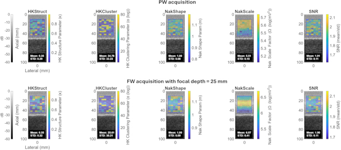
Figure 6. Envelope statistics parameter maps estimated for the 60 µm tissue-mimicking phantom. Quantitative ultrasound parameter maps obtained using (top) plane-wave (PW) acquisition and (bottom) focused-wave (FW) acquisition with a focal depth of 25 mm. Maps include the Homodyned-K structure parameter, Homodyned-K clustering parameter, Nakagami shape parameter, Nakagami scale parameter, and Rayleigh signal-to-noise ratio (SNR). Please click here to view a larger version of this figure.

The mean Nakagami scale parameter was 5.51 ± 0.15 and 6.07 ± 0.41 for PW and FW acquisition modes, respectively, reflecting the local backscattered signal energy within the ROI. Differences in the estimated scale parameter between acquisition modes are expected because of differences in the transmitted acoustic field, beamforming characteristics, and local signal intensity. For PW and FW acquisition modes, the mean H-K structure parameter was 0.35 ± 0.29 and 0.35 ± 0.32, respectively, whereas the mean H-K clustering parameter was 34.8 ± 33.2 and 25.6 ± 30.3, respectively. These large clustering parameter values, together with their large standard deviations, indicate unstable estimates for this phantom. As described in Protocol Steps 4.5.7–4.5.10, H-K parameter estimation relies on an iterative fitting procedure without a closed-form solution. When the fitting algorithm fails to converge, the estimated parameter values saturate and the fitting procedure terminates. Estimation failure is likely to occur for this phantom because the high scatterer number density and random spatial distribution of the glass beads produce scattering conditions approaching a fully developed Rayleigh regime, in which the H-K model has reduced sensitivity. In contrast, H-K parameter estimation has been reported to perform more reliably in biological tissue, where scattering conditions are more favorable for stable convergence³⁸. Overall, the Nakagami and Rayleigh SNR parameters obtained using both PW and FW acquisition modes were in close agreement, demonstrating consistent parameter estimation across the two acquisition configurations for these envelope statistics-based parameters.

ATS phantom validation of BSC-based mid-band fit and effective acoustic concentration parameters

To validate the MBF and EAC parameters, QUS processing was performed on an ATS tissue-mimicking phantom containing contrast targets with known relative backscatter levels using PW acquisition mode. A processing sub-ROI size of 4.1 mm (lateral) × 3 mm (axial) was used to ensure that each sub-ROI remained within the boundaries of an individual contrast target. Figure 7A shows the ATS phantom layout with the annotated contrast targets corresponding to relative backscatter levels of +3 dB, −3 dB, and −6 dB with respect to the surrounding background. The MBF parameter was estimated within each contrast target, yielding values of 4.60 dB, −1.37 dB, and −4.58 dB for the +3 dB, −3 dB, and −6 dB targets, respectively, as shown in Figure 7B. The corresponding relative differences in MBF between adjacent contrast targets were −5.97 dB and −3.21 dB, which closely matched the expected differences of −6 dB and −3 dB specified for the phantom. Similarly, the EAC parameter, obtained by Gaussian scattering model fitting of the estimated BSC, yielded values of 91.2 dB, 85.2 dB, and 82.1 dB for the +3 dB, −3 dB, and −6 dB targets, respectively, as shown in Figure 7C. The corresponding relative differences between adjacent targets were −6.05 dB and −3.09 dB, again closely matching the expected contrast differences. These results demonstrate that both MBF and EAC accurately capture relative differences in acoustic backscatter strength and support the ability of the pipeline to quantify acoustic contrast.

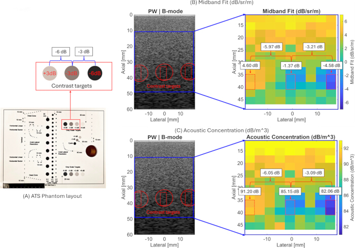
Figure 7. Quantitative ultrasound (QUS) parameter mapping of an ATS tissue-mimicking phantom. (A) Phantom layout highlighting the contrast targets. (B) Mid-band fit (MBF) parameter map. (C) Effective acoustic concentration (EAC) parameter map demonstrating differentiation of the +3 dB, −3 dB, and −6 dB contrast inclusions. Please click here to view a larger version of this figure.

QUS parameter maps of biological tissue

To demonstrate the applicability of the pipeline to biological tissue, the QUS imaging pipeline was applied to an ex vivo chicken breast sample. Figure 8 shows the estimated QUS parameter maps, including BSC-based parameters (ESD, EAC, MBF, SS, and I0), attenuation-based parameters (attenuation coefficient and attenuation intercept), and envelope statistics-based parameters (Nakagami shape and scale parameters and H-K structure and clustering parameters), overlaid on the corresponding B-mode images. Parameter estimation was performed over a 30 mm (lateral) × 27 mm (axial) ROI subdivided into 5 mm × 3 mm sliding sub-ROIs.

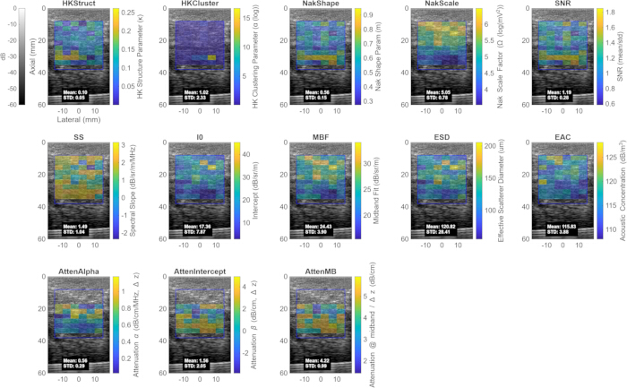
Figure 8. Quantitative ultrasound (QUS) parameter maps estimated from ex vivo chicken breast tissue. Envelope statistics-, attenuation-, and backscatter coefficient (BSC)-based parameter maps are displayed as color overlays on the corresponding B-mode images. The displayed parameters include the Homodyned-K structure parameter, Homodyned-K clustering parameter, Nakagami shape parameter, Nakagami scale parameter, Rayleigh signal-to-noise ratio (SNR), spectral slope (SS), spectral intercept (I0), mid-band fit (MBF), effective scatterer diameter (ESD), effective acoustic concentration (EAC), attenuation coefficient (AttenAlpha), attenuation intercept (AttenIntercept), and attenuation at the mid-band (AttenMB). Please click here to view a larger version of this figure.

The envelope statistics results showed a mean Nakagami shape parameter of 0.56 ± 0.15 and a Rayleigh SNR of 1.19 ± 0.28, indicating a deviation from fully developed Rayleigh speckle consistent with pre-Rayleigh scattering behavior expected from structurally heterogeneous biological tissue. The mean Nakagami scale parameter was 5.05 ± 0.78, reflecting the local backscattered signal energy within the ROI. The mean H-K structure parameter was 0.10 ± 0.05, and the mean H-K clustering parameter was 1.02 ± 2.33. The large spatial variability observed in the H-K clustering parameter likely reflects tissue heterogeneity.

The attenuation coefficient was estimated to be 0.56 ± 0.29 dB/cm/MHz, with an attenuation intercept of 1.56 ± 2.05 dB/cm. The relatively large variability in the attenuation intercept is expected because it is obtained by extrapolating the attenuation fit to 0 MHz, outside the measured processing bandwidth, making it sensitive to small variations in the estimated attenuation curve. In contrast, the attenuation within the processing bandwidth remained relatively stable, yielding a mean attenuation of 4.22 ± 0.99 dB/cm at the mid-band frequency of 4.75 MHz. Because Coila et al.³⁹ reported attenuation using a zero-intercept linear fit, comparison was performed using attenuation at the common mid-band frequency rather than the fitted slope and intercept parameters. Coila et al.³⁹ reported an attenuation coefficient of 0.83 ± 0.43 dB/cm/MHz for chicken breast tissue, corresponding to an attenuation of 3.94 dB/cm at 4.75 MHz. The estimated mid-band attenuation of 4.22 ± 0.99 dB/cm obtained in the present study is in good agreement with this value, with the observed differences likely attributable to variations in tissue preparation and estimation methodology.

The estimated attenuation coefficient and attenuation intercept were subsequently used as inputs to the reference phantom method for BSC estimation. The BSC-based linear fit parameters were estimated as follows: SS = 1.49 ± 1.04 dB/sr/m/MHz, I0 = 17.4 ± 7.87 dB/sr/m, and MBF = 24.4 ± 3.90 dB/sr/m. Gaussian scattering model fitting yielded an ESD of 121 ± 28.4 µm and an EAC of 115 ± 3.88 dB/m³.

These representative results demonstrate that the pipeline can generate a comprehensive set of QUS parameter maps and quantitative tissue descriptors from biological tissue using the integrated spectral-based, attenuation-based, and envelope statistics-based processing methods.

Performance metrics

Table 2 summarizes the processing frame rate for different QUS parameter configurations using both PW and FW acquisition modes (focal depth = 25 mm). The reported processing frame rates represent the end-to-end processing pipeline following beamformed RF acquisition, including data transfer, loading of the beamformed RF data, QUS computation, and display of the selected parameter map. Performance was evaluated over a 30 mm × 30 mm ROI with a scan depth of 55 mm. All measurements were obtained using a laptop equipped with an Intel Core Ultra 7 255H processor (20 cores, approximately 2.4 GHz) and 32 GB of RAM. Overall, the processing frame rate decreased as additional QUS parameters were selected for computation, consistent with the increased computational demand of each additional processing step.

Configuration		Parameters Computed				FPS (PW)	FPS (FW)
Envelope statistics only (Nakagami + Rayleigh SNR)		Nakagami shape, Nakagami scale, Rayleigh SNR				2.0	1.8
Envelope statistics only (all, including Homodyned-K)		Nakagami shape, Nakagami scale, Rayleigh SNR, Homodyned-K structure, Homodyned-K clustering				1.5	1.5
Backscatter coefficient (BSC)-based parameters only		Effective scatterer diameter (ESD), effective acoustic concentration (EAC), mid-band fit (MBF), spectral slope (SS), spectral intercept (I0)				0.8	0.8
Attenuation-based parameters only		Attenuation coefficient (AttenAlpha), attenuation intercept (AttenIntercept), attenuation at the mid-band (AttenMB)				0.8	0.8
Envelope statistics (excluding Homodyned-K) + BSC-based parameters		Nakagami shape, Nakagami scale, Rayleigh SNR, ESD, EAC, MBF, SS, I0				0.7	0.7
All parameters (excluding Homodyned-K)		Nakagami shape, Nakagami scale, Rayleigh SNR, ESD, EAC, MBF, SS, I0, AttenAlpha, AttenIntercept, AttenMB				0.4	0.4
All parameters		Nakagami shape, Nakagami scale, Rayleigh SNR, Homodyned-K structure, Homodyned-K clustering, ESD, EAC, MBF, SS, I0, AttenAlpha, AttenIntercept, AttenMB				0.4	0.4

Table 2: Processing frame rate (frames per second [FPS]) for different quantitative ultrasound (QUS) parameter configurations over an imaging depth of 10–40 mm using 5 mm × 3 mm sliding sub-regions of interest (sub-ROIs). Processing performance is reported for plane-wave (PW) and focused-wave (FW) acquisition modes using different combinations of envelope statistics-, backscatter coefficient (BSC)-based, and attenuation-based QUS parameters.

As summarized in Table 2, envelope statistics-based processing alone, consisting of Nakagami fitting and Rayleigh SNR estimation, yielded the highest frame rates of 2.0 frames/s and 1.8 frames/s for PW and FW acquisition modes, respectively. Adding H-K parameter estimation reduced the processing frame rate to 1.5 frames/s for both acquisition modes, reflecting the higher computational cost of iterative H-K fitting. Independently computing either BSC-based parameters or attenuation-based parameters resulted in frame rates of approximately 0.8 frames/s for both PW and FW acquisition modes. Combining envelope statistics-based parameters (excluding H-K) with BSC-based parameters further reduced the processing frame rate to 0.7 frames/s.

Computing all implemented parameters except H-K yielded a processing frame rate of 0.4 frames/s. When H-K fitting was included together with all other parameters, a frame rate of approximately 0.4 frames/s was achieved for the tissue-mimicking phantoms evaluated in this study. The processing time required for H-K fitting depended on the imaging medium. Media exhibiting nearly homogeneous scattering or air-like scattering properties required additional iterations for convergence of the iterative H-K fitting algorithm, resulting in frame rates below 0.4 frames/s.

These results demonstrate the trade-off between processing speed and the number of QUS parameters computed. For near real-time imaging applications, combining envelope statistics-based parameters (excluding H-K) with BSC-based parameters provided a practical balance between parameter diversity and computational performance, achieving a processing frame rate of approximately 0.7 frames/s. H-K parameter estimation is therefore better suited for offline analysis or applications in which higher temporal resolution is not required.

Обсуждение

This paper describes a QUS processing pipeline with a user-friendly numerical computing software–based GUI implemented on an ultra-portable USB-C-connected ultrasound system. The pipeline integrates spectral-based BSC and attenuation estimation, model-based parameter extraction, and envelope statistics-based parameter estimation to provide multiple complementary quantitative descriptors of tissue microstructure. The reference phantom method used for BSC and attenuation estimation, together with Gaussian scattering model fitting and envelope statistics analysis, builds upon established quantitative ultrasound methodologies for tissue characterization^{4,5,6,16,17,25,26,29}. Validation using tissue-mimicking phantoms demonstrated that the estimated BSC curves and derived BSC-based parameters were in close agreement with theoretical predictions for both PW and FW acquisition modes (Table 1). In particular, the mean mid-band BSC estimates remained within 0.5 dB of the theoretical value obtained using Faran scattering theory, while temporal averaging over 20 frames substantially reduced estimation variability without introducing systematic bias. Similarly, the estimated ESD, EAC, SS, I0, and MBF remained close to their expected theoretical values (Table 1). The estimated Nakagami shape parameter and Rayleigh SNR were also consistent with the fully developed speckle expected from a dense random scatterer distribution, supporting the validity of the implemented envelope statistics-based processing pipeline^16,18,34,37. Furthermore, attenuation estimates obtained from ex vivo chicken breast tissue agreed with previously reported values³⁹, while the ATS phantom experiments demonstrated that MBF and EAC accurately quantified relative differences in acoustic backscatter strength. The H-K distribution parameters further complemented tissue characterization by providing information related to heterogeneous scattering environments, consistent with previous reports demonstrating their utility for biological tissue characterization and classification^17,19,34,38. Collectively, these findings support the proposed pipeline as a validated framework for quantitative point-of-care ultrasound imaging capable of generating complementary quantitative information beyond conventional B-mode imaging.

Several critical steps in the protocol require particular attention to ensure reproducible QUS parameter estimation. Accurate attenuation compensation is essential for unbiased BSC estimation because incorrect attenuation values introduce systematic depth-dependent bias into the estimated BSC and derived parameters^25,26,29. When the attenuation properties of the imaging medium are not known a priori, an initial estimate can be obtained using the pipeline’s built-in total attenuation estimation functionality and subsequently used to compensate attenuation effects during BSC computation (Equation 1). Because attenuation is estimated relative to the initial sub-ROI, this reference sub-ROI should be positioned close to the probe surface while remaining sufficiently deep to avoid near-field effects. The processing bandwidth should also be carefully selected to match the usable frequency range of both the sample and reference phantom RF power spectra. The recommended approach is to use the common −6 dB bandwidth of the reference phantom power spectrum. For the ultrasound probe used in this study, the recommended processing bandwidth is 3–6.5 MHz. Users should verify that the selected bandwidth corresponds to the overlapping spectral region in which both the sample and reference spectra remain within 6 dB of their peak power, thereby restricting BSC and attenuation estimation to the high-SNR region and minimizing the influence of system noise^6,25,26. In addition, accurate BSC estimation using the reference phantom method requires the probe to be maintained approximately perpendicular to the phantom or tissue surface, consistent with the scan geometry used during acquisition of the reference phantom dataset²⁵.

The current implementation has several limitations that should be considered when applying the protocol. Under near real-time operating conditions, single-frame BSC-based parameter estimation exhibits relatively high variability because model-based spectral fitting is inherently sensitive to fluctuations in the estimated power spectra arising from measurement noise and speckle variability^4,5,6. The spatial resolution of the QUS parameter maps is also limited by the selected sub-ROI dimensions. Smaller sub-ROIs improve spatial resolution but reduce the number of independent samples available for spectral and statistical fitting, thereby increasing estimation variability, whereas larger sub-ROIs improve estimation stability at the expense of spatial resolution^40,41,42. The current implementation is further limited to an imaging depth of approximately 5 cm because the available reference phantom RF dataset extends only over this depth range; imaging deeper structures therefore requires acquisition of additional reference phantom data. Finally, the current implementation exports RF data as “.mat” files, which limits data transfer efficiency between the probe and the laptop. IQ-domain QUS processing has been shown to reduce computational cost and memory usage while maintaining comparable spectral-based QUS performance⁴³; however, the current ultrasound platform provides access only to beamformed RF data and does not output beamformed IQ data. As summarized in Table 2, combining envelope statistics-based parameters excluding H-K fitting with BSC-based parameters provided a practical balance between parameter diversity and computational performance, achieving a processing rate of approximately 0.7 frames/s for near real-time imaging. Because H-K parameter estimation is computationally intensive and relies on iterative optimization without a closed-form solution^17,34, it is better suited for offline analysis or applications in which higher temporal resolution is not required.

Several opportunities exist to further extend the capabilities of the current pipeline. To reduce parameter variability under near real-time operating conditions, future updates will incorporate multi-frame averaging of consecutive RF acquisitions before QUS parameter estimation, thereby reducing electronic noise and stochastic spectral fluctuations arising from speckle variability while maintaining near real-time operation. Here, the term “near real-time” refers to interactive QUS parameter estimation and visualization during image acquisition rather than conventional offline post-processing. Although the achievable frame rate decreases for more computationally demanding QUS parameters, particularly BSC- and attenuation-based processing and H-K estimation, these parameters characterize tissue properties that are not expected to change rapidly during scanning. Therefore, near real-time operation is primarily intended to provide timely feedback for probe positioning, ROI selection, and processing parameter adjustment rather than to capture dynamic physiological changes. Future work will investigate the integration of regularized QUS estimation methods^40,41,42. These approaches may enable increased sub-ROI overlap during QUS estimation, thereby improving the spatial resolution of QUS parameter maps while maintaining practical near real-time performance. More computationally efficient methods for H-K parameter estimation, including table-search and artificial neural network-based estimators^35,36, will also be investigated to reduce computation time on the ultrasound platform. In addition, reference-free QUS methods for attenuation estimation⁴⁴ will be investigated to reduce dependence on reference phantom acquisitions and further simplify the clinical workflow. Because QUS parameter estimation is performed independently for each sub-ROI, the computational workload is inherently parallelizable and well suited for GPU implementation. Processing speed optimization was not a primary objective of the present study; therefore, future versions will incorporate GPU-accelerated QUS processing⁴⁵ together with additional code optimization to improve processing speed, facilitate higher frame rates, and enable more efficient multi-frame averaging.

Although the present pipeline was validated using the ultrasound probe and acquisition configurations described in this protocol, the modular processing framework can be adapted to other ultrasound probes and imaging sequences by updating the acquisition configuration and corresponding reference phantom dataset. Extension to another scanner requires access to suitable RF or IQ data, adaptation of the data acquisition and import interfaces to the platform-specific software development kit or RF data format, and acquisition of appropriate reference phantom data for the intended imaging configurations. The current software depends on a proprietary MEX interface required for data acquisition and processing on the ultrasound platform and therefore cannot currently be released as a standalone public package. Nevertheless, the processing framework is modular, and the individual analysis stages can be separated conceptually from the platform-specific acquisition interface. This design provides a practical path for future adaptation to platforms that expose raw RF, beamformed RF, or IQ data through different software interfaces. Future work will also expand the range of supported QUS parameters to include entropy- and multiple scattering-based metrics, as well as investigate deep learning-based tissue classification using multiparametric QUS maps as imaging biomarkers, building on previous studies demonstrating the feasibility of QUS-based tissue characterization and classification^{7,11,12,13,14,20,21}.

The significance of this work lies in providing a comprehensive QUS processing pipeline for an ultra-portable ultrasound platform that can be deployed beyond traditional research laboratories and conventional cart-based ultrasound systems. Although handheld ultrasound devices have become increasingly available for point-of-care imaging^22,23, most quantitative ultrasound implementations continue to rely on research scanners or cart-based systems^8,9,10,11,24. By integrating spectral-, attenuation-, and envelope statistics-based QUS analysis within a user-friendly numerical computing software–based GUI requiring no specialized programming expertise, the present pipeline lowers the technical barrier to performing quantitative ultrasound tissue characterization on a portable platform. The modular framework further facilitates adaptation to different probes, acquisition schemes, and research applications, supporting translational quantitative ultrasound studies across a broad range of preclinical and clinical imaging applications^{7,8,9,10,11,12,13,14,20,21,24}. This balance is important for point-of-care use, where computational efficiency, reproducibility, and ease of operation must be considered together with quantitative accuracy. The present implementation therefore emphasizes an integrated workflow rather than acceleration of a single processing stage, while preserving access to the underlying RF data and allowing users to modify processing parameters according to the intended application. Although additional optimization and broader platform validation are required before routine clinical deployment, the present work establishes a practical implementation pathway for bringing multiparametric QUS analysis closer to point-of-care use while preserving the quantitative information available from spectral and envelope statistics-based methods.

Материалы

Список материалов, использованных в этой статье

Имя	Компания	Каталожный номер	Комментарии
18 μm tissue-mimicking phantom	University of Wisconsin Madison	Not applicable	Agar-based tissue-mimicking phantom containing 18.2 μm borosilicate glass bead scatterers; used as sample/reference phantom as applicable.
60 μm tissue-mimicking phantom	University of Wisconsin Madison	Not applicable	Agar-based tissue-mimicking phantom containing 60 μm borosilicate glass bead scatterers.
BufferData MATLAB file	Not applicable	Not applicable	Exported .mat file generated by the GUI and loaded for offline visualization and reprocessing.
DKPOC LA 6.0 128 2433 linear ultrasound transducer	Vermon SA, Tours, France	029076 - DKPOC - LA 6.0 128 -2423	Linear 128-element ultrasound transducer.
GUI_v1_main1.m script	Not applicable	Not applicable	MATLAB script used to initialize the ultrasound system and launch the graphical user interface.
Laptop computer	Lenovo Group Ltd., Beijing, China	Lenovo Legion 5 15IAX10	Laptop used to run MATLAB and interface with the ultrasound probe.
load_saved_data.m script	Not applicable	Not applicable	MATLAB script used for offline visualization and reprocessing of saved RF data and QUS parameter maps.
MATLAB	The MathWorks, Inc.	MATLAB 2025b (Signal Processing, Statistics and Machine Learning abd Curve Fitting toolboxes)	Programming and numerical computing environment; manuscript states version 2018a or later.
Reference phantom membrane material	Mitsui Chemicals, Rye Brook, NY, USA	Not applicable	TPX/polymethylpentene membrane, 25 μm thick.
The OPTIMAL phantom	Sonora Medical Systems, USA	Not applicable	Tissue-mimicking phantom containing contrast targets.
USB-C cable	Permanently connected to the transducer	Not applicable	Cable used to connect the ultrasound probe to the laptop through a Thunderbolt-compatible USB-C port.