A Comparative Evaluation of YOLO-Segmentation Models for Coronary Artery Segmentation on the ARCADE Dataset

Краткое содержание

This protocol presents a reproducible image-level comparison of five YOLO-segmentation models for coronary artery segmentation on the public ARCADE X-ray angiography dataset. It is for methodological benchmarking, not clinical validation. Latency–accuracy trade-offs require prospective, hardware-specific validation.

Аннотация

Coronary X-ray angiography is the clinical reference for visualizing coronary anatomy, but automated instance-level segment labeling remains difficult because of low contrast, overlapping branches, class imbalance across 25 SYNTAX-defined segments, and heterogeneous published protocols. This protocol therefore provides a reproducible, image-level comparison of five You Only Look Once (YOLO) segmentation models—YOLOv8-seg, YOLOv9c-seg, YOLO11-seg, YOLO12-seg, and YOLO26-seg—on the public Roboflow v1 ARCADE release of 3,587 expert-annotated frames divided into 3,138 training, 299 validation, and 150 test frames. Models were initialized from official segmentation checkpoints, trained only on the training split with shared stochastic gradient descent (SGD) settings and validation-based early stopping and checkpoint selection, and evaluated once post hoc on the untouched test split; mask mean average precision (mAP) at intersection over union (IoU) thresholds of 0.50–0.95 (mAP@50–95) was the primary accuracy metric and A100 model-level latency at 32-bit floating-point precision (FP32) was a secondary efficiency descriptor. On validation, the larger YOLOv9c-seg obtained the highest observed mask mAP@50–95 of 0.210; on the test split, compact YOLO11-seg obtained the highest observed mask mAP@50–95 of 0.241, followed by YOLO26-seg (0.239) and YOLOv9c-seg (0.235). Major proximal segments were consistently easier to segment than rare distal variants, while recorded inference times of 0.6 ms versus 3.0 ms per frame describe model-level throughput rather than end-to-end clinical latency. These single-seed, image-level results do not establish patient-level independence, statistical superiority, or clinical utility; they are intended as a methodological benchmark that others can reimplement, with prospective, hardware-specific, and patient-level validation still required before any workflow claim.

Введение

Coronary artery disease (CAD) remains a major cause of global mortality. The World Health Organization fact sheet dated 31 July 2025 reports an estimated 19.8 million cardiovascular-disease deaths in 2022, approximately 32% of global deaths¹. Atherosclerotic plaque formation and progression involve interacting lipid, inflammatory, endothelial, and vascular-remodeling processes². Invasive X-ray coronary angiography provides real-time visualization of coronary anatomy and stenosis, but manual image interpretation and delineation can be time-consuming and observer-dependent³.

Deep learning is widely used for medical-image segmentation. U-Net and related encoder–decoder networks remain common biomedical baselines^4,5, including volumetric extensions such as 3D U-Net⁶. Semantic segmentation assigns a class to each pixel, object detection primarily localizes instances⁷, and instance segmentation additionally returns a separate mask for each annotated object. This distinction matters when adjacent coronary branches overlap or when a vessel boundary is required in addition to a box. YOLO-based instance segmentation predicts locations, classes, and masks in one forward pass⁷. Because published studies differ in datasets, labels, metrics, preprocessing, and hardware, the present work benchmarks YOLO-segmentation models and does not claim universal superiority over semantic segmentation or detection.

The YOLO family has been extended through successive detectors. YOLOv4 introduced architectural changes intended to improve speed and accuracy⁸. YOLOv7 later described trainable bag-of-freebies methods for real-time detection⁹. Ultralytics provides a unified implementation that supports detection and segmentation training¹⁰. YOLOv9 introduced programmable gradient information; its primary source supports the architecture and general detection benchmarks rather than a medical-segmentation result¹¹. A systematic review of deep-learning coronary-artery segmentation and CAD detection reports substantial heterogeneity in datasets, annotations, metrics, and study designs, which limits direct cross-study comparison¹².

Recent X-ray angiography studies illustrate that setting. Some report original models on private or modest cohorts and evaluate one architecture at a time^13,14. Reviews of YOLO in medical imaging show that many applications emphasize detection rather than pixel-level segmentation^15,16. These reviews motivate a transparent, head-to-head comparison on a documented public split, not a claim that YOLO is preferable to U-Net-style baselines.

Public datasets and explicit split manifests improve reproducibility^17,18. Large public corpora in other imaging domains, including MIMIC-CXR, PASCAL VOC, MS COCO, and ImageNet, likewise document dataset composition and official splits^19,20,21,22. An image-level split still does not certify patient-level independence. This study uses the Roboflow v1 release of the public ARCADE dataset, which contains 3,587 expert-labeled X-ray coronary angiography images, annotations for 25 coronary segments, and a predefined train/validation/test split of 3,138/299/150 images¹⁷. The available source materials do not report the number of unique patients, the number of angiographic sequences or views per patient, an annotator count, inter-annotator agreement, or a patient-level manifest, and they do not state whether frames from one patient can appear in more than one subset. These items are treated as limitations.

Artificial intelligence may eventually support clinical imaging workflows, but integration requires standardized data representation, transparent evaluation, and prospective validation^23,24. Cross-validation and bootstrap methods are useful statistical tools for accuracy estimation; they are not a universal clinical gold standard²⁵. Batch normalization is a common training component²⁶. Contrast-limited adaptive histogram equalization, image augmentation, compact MobileNets backbones, and transfer learning are relevant methodological concepts^27,28,29,30. Standard deep-learning practice is summarized in established textbooks³¹. Compact feature extractors and anchor-free detectors in aerial imagery provide architectural context rather than an ARCADE baseline^32,33,34. Related medical segmentation modules outside angiography are cited on the same basis³⁵. Real-time YOLO detection and instance-segmentation pipelines in agricultural imaging are likewise treated as implementation context, not as numerical comparators^{36,37,38,39,40,41,42}.

This study presents a methodological comparison of five YOLO-segmentation models on the public ARCADE dataset. The contributions are: (1) a reproducible image-level train/validation/test protocol; (2) a head-to-head comparison of five YOLO-segmentation variants; (3) analysis of architecture size, class-wise behavior, and documented failure modes; and (4) a descriptive comparison of accuracy and throughput that is separated from clinical validation.

Протокол

This investigation is a secondary analysis of openly accessible, de-identified ARCADE data. Do not recruit participants or acquire new clinical images for this protocol. The original ARCADE source reported its own ethics and consent procedures; this secondary analysis does not replace those procedures. Use the materials listed in the Table of Materials.

1. Dataset preparation

1. Download the ARCADE dataset from the official ARCADE source or the Roboflow project project-5ykjl/arcade-swkv3, version 1, released 12 March 2025.
2. Confirm that the export contains 3,587 X-ray coronary angiography images with expert annotations and the image-level split 3,138 train / 299 valid / 150 test.
3. Record the Roboflow v1 export preprocessing as Auto-Orient and stretch to 640 × 640 pixels.
4. Inspect the available manifest for patient identifiers, sequence identifiers, view identifiers, and frame-overlap checks.
5. If starting from raw Digital Imaging and Communications in Medicine (DICOM) files, convert each image to 8-bit PNG at 640 × 640 pixels. If using the Roboflow export, use the supplied PNG files and do not repeat this conversion.
6. Organize the dataset as images/train/, images/valid/, images/test/, labels/train/, labels/valid/, and labels/test/. Store one label file per image containing the class index and polygon coordinates.
   NOTE: The supplied materials document the image-level 3,138/299/150 split but do not certify patient-level separation, unique patient counts, sequences or views per patient, annotator count, or inter-annotator agreement. Conversion to 8-bit PNG discards original intensity precision and DICOM physical metadata.

2. Data preprocessing

1. Verify that exported images are Auto-Oriented and stretched to 640 × 640 pixels.
2. Do not apply an extra normalization or contrast-enhancement step unless that step is recorded and applied identically to every split.
3. Keep validation and test images unaugmented.
4. Do not move images between train, valid, and test.
   CAUTION: If any additional intensity or geometric transform is added later, inspect transformed angiograms for anatomically implausible changes before accepting the run.

3. Model implementation

1. Obtain the five pretrained segmentation checkpoints: yolov8n-seg.pt, yolov9c-seg.pt, yolo11n-seg.pt, yolo12n-seg.pt, and yolo26n-seg.pt.
2. Load each model from its .pt checkpoint. Do not treat an architecture YAML file alone as evidence of pretrained-weight loading.
3. Set the output layer to 25 coronary-artery classes and verify the class-name order against data.yaml.
4. Record implementation provenance before training:
   1. Use Ultralytics as the source package for YOLOv8-seg, YOLO11-seg, YOLO12-seg, and YOLO26-seg.
   2. Use the WongKinYiu/yolov9 repository as the source attribution for YOLOv9c-seg.
   3. Record the package version, checkpoint filename, and, if available, the repository commit and checkpoint hash.
      NOTE: Exact repository commits and checkpoint hashes were not retained for the reported runs. YOLOv9c-seg is materially larger than the other four models, so the comparison is not size-matched.

4. Model training

1. Set the training environment to Ultralytics 8.4.51, PyTorch 2.10.0, CUDA 12.8, Python 3.12.13, and an NVIDIA A100-SXM4-40GB graphics processing unit (GPU).
2. Set shared baseline hyperparameters:
   1. Set the optimizer to SGD, momentum to 0.9, initial learning rate to 0.01, and weight decay to 0.00005.
   2. Set the image size to 640 pixels, random seed to 0, maximum number of epochs to 600, and early-stopping patience to 30 epochs.
   3. Use the default Ultralytics segmentation loss, comprising box, segmentation, classification, and distribution-focal terms.
3. Use these effective batch sizes: 128 for YOLOv8-seg; 32 for YOLOv9c-seg after memory reduction; 128 for YOLO11-seg; 128 for YOLO12-seg; 128 for YOLO26-seg.
4. Apply training-time augmentation only to the training split. Do not override Ultralytics augmentation arguments unless a new run is being documented. For Ultralytics 8.4.51, use the package default settings:
   1. Set hsv_h=0.015, hsv_s=0.7, hsv_v=0.4.
   2. Set degrees=0.0, translate=0.1, scale=0.5, shear=0.0, perspective=0.0.
   3. Set flipud=0.0, fliplr=0.5, bgr=0.0.
   4. Set mosaic=1.0, mixup=0.0, copy_paste=0.0, close_mosaic=10.
5. Train each model on the 3,138-image training split.
6. Use the 299-image validation split only for validation fitness, early stopping, and checkpoint selection. Do not use the test split during training or model selection.
7. Save the checkpoint with the best validation fitness. Save the run folder files, including args.yaml, the checkpoint path, and the completed epoch count.
8. After checkpoint selection, load the selected checkpoint and evaluate it on the 150-image test split.
   NOTE: The reported post hoc test evaluation used Ultralytics 8.4.157 on a Tesla T4.
9. Record training and validation loss, precision, recall, mAP@50, and mAP@50–95 at each epoch.
10. If measuring inference time, record the warm-up count, number of timed repetitions, timing batch size, numerical precision (e.g., FP32), and summary statistic.
    NOTE: Completed runs lasted approximately 63–121 epochs because early stopping used a patience of 30 epochs. The A100 measurements in Table 1 and the T4 test log in Table 2 are different environments; do not substitute T4 timing for Table 1. Timing-repetition details were not retained for the reported A100 values.

5. Reproducibility commands

1. Replace the checkpoint name, batch size, and run name for each model. Keep the explicit .pt argument.
   from ultralytics import YOLO
   model = YOLO('yolo26n-seg.pt')
   model.train(
   data='data.yaml',
   epochs=600,
   patience=30,
   batch=128, # use 32 for YOLOv9c-seg
   imgsz=640,
   seed=0,
   optimizer='SGD',
   lr0=0.01,
   momentum=0.9,
   weight_decay=5e-5,
   pretrained=True,
   task='segment',
   name='arcade_yolo26_seg'
   )
   model.val(data='data.yaml', split='val', imgsz=640, batch=1)
   model.val(data='data.yaml', split='test', imgsz=640, batch=1) # post hoc only
   model.predict(source='path/to/one_image.png', imgsz=640, conf=0.25, save=True, save_txt=True)
2. For YOLOv9c-seg, set batch=32 and YOLO('yolov9c-seg.pt'). For the other four models, set batch=128 and the corresponding *n-seg.pt checkpoint.

Результаты

This section reports the image-level outcomes of five YOLO-based instance-segmentation frameworks on the ARCADE benchmark. Validation results are reported in Table 3 and Table 4, and supplied post hoc test results are reported in Table 2. The image-level split should not be interpreted as a certified patient-level split.

Dataset characteristics

Figure 1A shows the instance counts for the 25 anatomical classes, and Figure 1B shows an overlay of normalized bounding boxes in the ARCADE dataset. Figure 1C,D show the distributions of bounding-box center coordinates and dimensions, respectively.

Architectural comparison

Table 5 summarizes the architectural specifications of the five evaluated YOLO-segmentation variants. YOLOv9c-seg is substantially larger than the other models, with 27.6 million parameters and 147.7 GFLOPs. The comparison, therefore, benchmarks recent implementations rather than strictly size-matched networks.

Training dynamics

Figure 2A shows the training and validation curves for YOLOv8-seg over 121 epochs. Figure 2B shows the training dynamics of YOLOv9c-seg, which reached early stopping at epoch 63. Figure 2C presents the curves for YOLO11-seg over 104 epochs. YOLO12-seg (Figure 2D) and YOLO26-seg (Figure 2E) completed 87 and 118 epochs, respectively. The curves describe training and validation optimization and are not used to rank models.

Figure 3 shows annotated training-batch samples, including ground-truth boxes, masks, and class names across several angiographic views. The panels illustrate label placement on overlapping branches, bifurcations, and segments with uneven contrast. Because these overlays are training annotations, they are not used as evidence of model predictions.

Figure 4 shows validation-batch frames with colored boxes, masks, and numeric class indices. Overlapping boxes and small or low-contrast segments are visible in several tiles. Quantitative comparison of models on these cases is reported in Table 3, Table 4, and Table 2 and in the confusion matrices in Figure 5A–E, rather than by visual inspection of individual tiles.

Segmentation performance

Table 3 summarizes the overall performance of all five models on the ARCADE validation set (n = 299). YOLOv9c-seg attained the highest observed validation mask mAP@50–95 of 0.210. These values are validation results used during model development and should not be treated as unbiased external-test estimates.

Figure 6A presents the box precision–recall curve for YOLOv9c-seg. Per-class box mAP@50 ranged from 0.013 to 0.879, with higher scores on major segments (class 1: 0.618; class 11: 0.726; class 5: 0.828) and lower scores on rare or distal labels (class 10a: 0.013; class 12: 0.113; class 16c: 0.169). Figure 6B shows the corresponding mask curve, with mask mAP@50 from 0.000 to 0.884. Figure 6C,D display the box and mask curves for YOLOv8-seg; mask mAP@50 exceeded 0.70 for classes 1, 2, 3, 5, and 11. Figure 6E and Figure 7A present the box and mask curves for YOLO11-seg, respectively. Figure 7B,C present the box and mask curves for YOLO12-seg, respectively, and Figure 7D,E present the corresponding curves for YOLO26-seg. The same major-versus-rare gradient appears across architectures.

Per-class segmentation analysis

Table 4 reports per-class mask mAP@50 and mAP@50–95 for all five models. Major segments generally score higher than rare variants and small branches. Figure 1A shows 15 instances for class 10a in the displayed dataset-wide count; a split-specific count for train, validation, or test was not tabulated separately. The default Ultralytics loss did not include an explicit rare-class weight.

Four error types can be separated with the available metrics, without assigning unverified case identifiers. Missed detections correspond to low recall and low precision–recall curves for sparse labels such as 10a, 12, and 16c in Figure 6A–E and Figure 7A–E. Incorrect class assignment and adjacent-class confusion appear as off-diagonal entries in Figure 5A–E, especially between 12a/12b and 16a/16b/16c. Boundary inaccuracy is only indirectly indicated by the gap between box and mask mAP in Table 3 and Table 4; Dice, IoU, and contour-distance values were not computed. Low contrast and overlap are visible as label crowding in Figure 3 and Figure 4, but those panels are not used to rank models.

Figure 5A presents the normalized confusion matrix for YOLOv8-seg. Figure 5B–E present the matrices for YOLOv9c-seg, YOLO11-seg, YOLO12-seg, and YOLO26-seg, respectively. Major classes 1, 2, 3, 5, and 11 show stronger diagonal dominance than the small-branch labels. Background assignment is more frequent for the smaller segments.

Figure 8A shows training visualizations for YOLOv8-seg over 121 epochs. Figure 8B–E show the corresponding plots for YOLOv9c-seg, YOLO11-seg, YOLO12-seg, and YOLO26-seg, respectively. Training loss decreases in all runs. Several validation-loss curves plateau or separate from training loss, so the plots do not support a uniform claim of closely aligned curves or minimal overfitting. Use Figure 8A–E together with Figure 2A–E as a description of convergence, not as proof of generalization.

Computational efficiency

Table 1 reports model-level GPU inference time and training characteristics on the A100/FP32 setup. These values exclude data loading, host–device transfer, mask decoding, post-processing, display, and clinical workflow steps, and they are not end-to-end latency. YOLOv8-seg and YOLO11-seg recorded 0.6 ms per frame; YOLOv9c-seg recorded 3.0 ms. The timing record does not include the number of warm-up runs, the number of timed repetitions, the timing batch size, or whether each value is a mean, median, or minimum. Compact models were smaller than 7 MB; YOLOv9c-seg was 56.3 MB.

The compact variants had model sizes below 7 MB, whereas YOLOv9c-seg was 56.3 MB. Training duration and peak GPU memory are also hardware- and batch-size-dependent. These A100 measurements indicate model-level computational behavior under the reported setup, not guaranteed performance on clinical workstations or edge devices.

Comparison with existing methods

Published U-Net and other segmentation results use different datasets, labels, metrics, preprocessing, and hardware, so their Dice values and timing cannot be directly compared with the present YOLO mAP values. A same-dataset, same-protocol U-Net or nnU-Net baseline remains necessary for a fair accuracy-efficiency comparison.

On the validation split, YOLOv9c-seg had the highest observed mask mAP@50–95 (0.210). On the untouched test split, YOLO11-seg had the highest observed mask mAP@50–95 (0.241), followed by YOLO26-seg (0.239) and YOLOv9c-seg (0.235). These single-seed results are descriptive only. No composite speed–accuracy score was defined, so the study does not identify a formally optimal model. The A100 measurements indicate that YOLO11-seg is smaller and faster than YOLOv9c-seg, while YOLOv9c-seg has higher validation mask mAP@50–95 and larger capacity.

The A100 timing values in Table 1 and the T4 evaluation log in Table 2 were produced under different environments and should not be compared as a hardware-independent speed ranking. Full pipeline timing, repeated seeds, confidence intervals, and patient-level external testing remain necessary before deployment claims can be made.

The source data are from the public ARCADE Challenge/Roboflow v1 release (project-5ykjl/arcade-swkv3, version 1; 3,587 images with 3,138/299/150 train/valid/test splits). The study-generated materials accompanying the revision include the split manifest, YOLO conversion configuration, numerical source data, test evaluation log, table workbooks, training logs, and model checkpoints, with redistribution permitted. The original images are not redistributed in this manuscript.

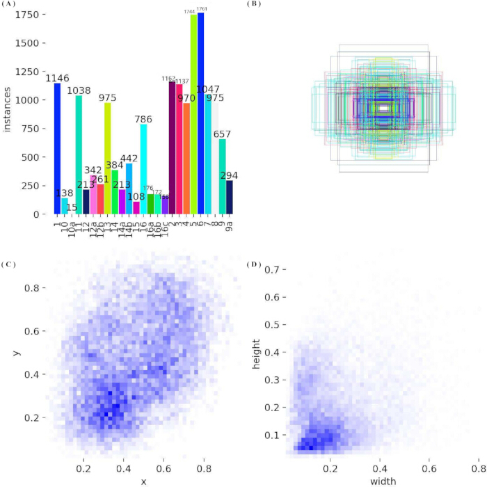
Figure 1: Distribution of bounding boxes in the ARCADE dataset. (A) Instance counts for all 25 anatomical classes, from left to right: 1 (1146), 10 (138), 10a (15), 11 (1038), 12 (213), 12a (342), 12b (261), 13 (975), 14 (384), 14a (213), 14b (442), 15 (108), 16 (786), 16a (176), 16b (172), 16c (158), 2 (1163), 3 (1137), 4 (970), 5 (1744), 6 (1761), 7 (1047), 8 (975), 9 (657), and 9a (294). (B) Overlay of normalized bounding boxes, which cluster near the frame center and vary in aspect ratio. (C) Binned density map of box-center coordinates (x, y), with higher density in the lower-central and upper-right regions of the frame. (D) Binned density map of normalized width versus height, showing that most boxes are elongated (height greater than width), consistent with tubular coronary segments. Please click here to view a larger version of this figure.

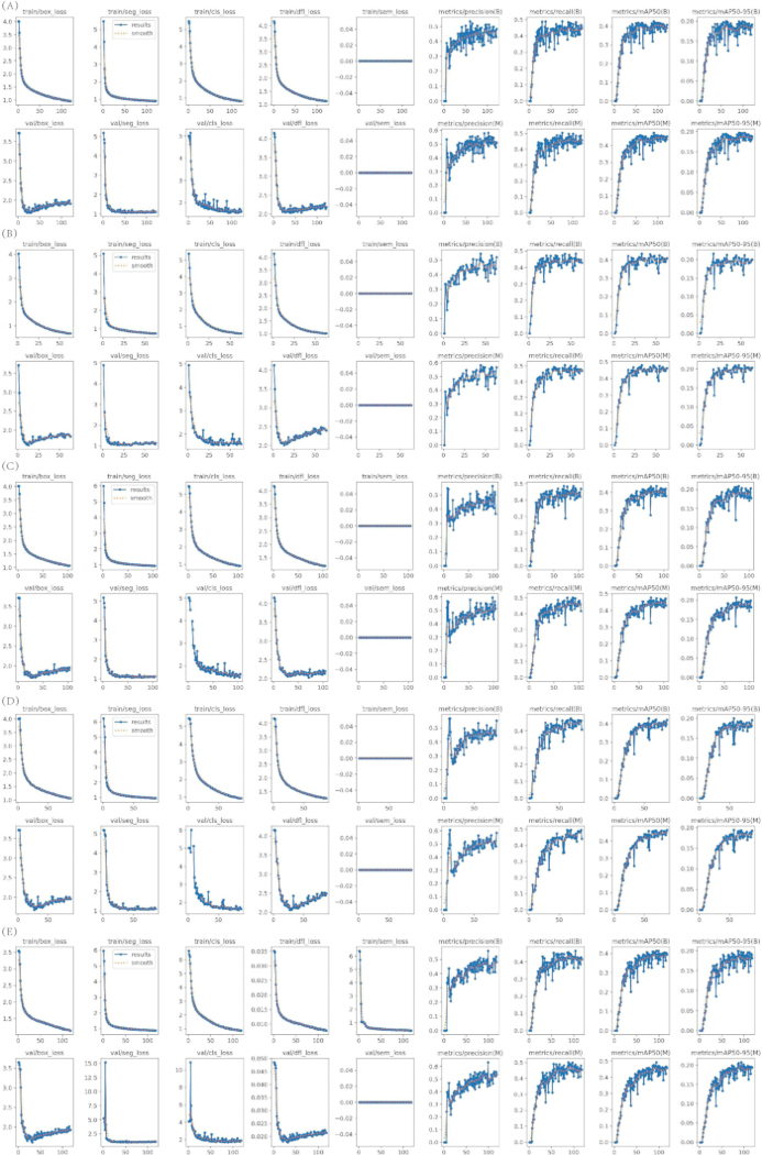
Figure 2: Training and validation curves for five YOLO segmentation models. (A) YOLOv8-seg (121 epochs). (B) YOLOv9c-seg (63 epochs). (C) YOLO11-seg (104 epochs). (D) YOLO12-seg (87 epochs). (E) YOLO26-seg (118 epochs). Each lettered block occupies two rows: the upper row shows training losses (box, segmentation, classification, distribution-focal, and semantic) and bounding-box metrics (precision, recall, mAP@50, and mAP@50–95); the lower row shows the corresponding validation losses and mask metrics. All curves are from a single run and are presented descriptively. Please click here to view a larger version of this figure.

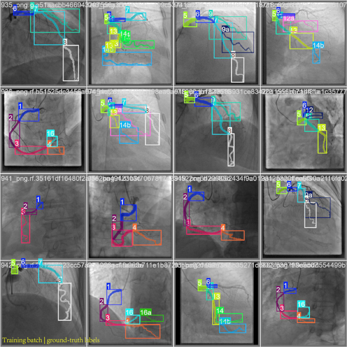
Figure 3: Annotated training-batch samples from the YOLO26-seg run on the ARCADE dataset. The on-figure title reads “Training batch | ground-truth labels.” The 4 × 4 mosaic is the Ultralytics training-batch view from this run. In each tile, colored rectangles are ground-truth bounding boxes, matching colored contours are ground-truth segmentation masks, and the text labels are SYNTAX segment names (for example, 1, 5, 9a, 14b, and 16a). Overlapping boxes mark adjacent or bifurcating branches in the same field of view. These overlays are trainer-supplied annotations from the YOLO26-seg training batches, not model predictions and not outputs from the other four architectures. Please click here to view a larger version of this figure.

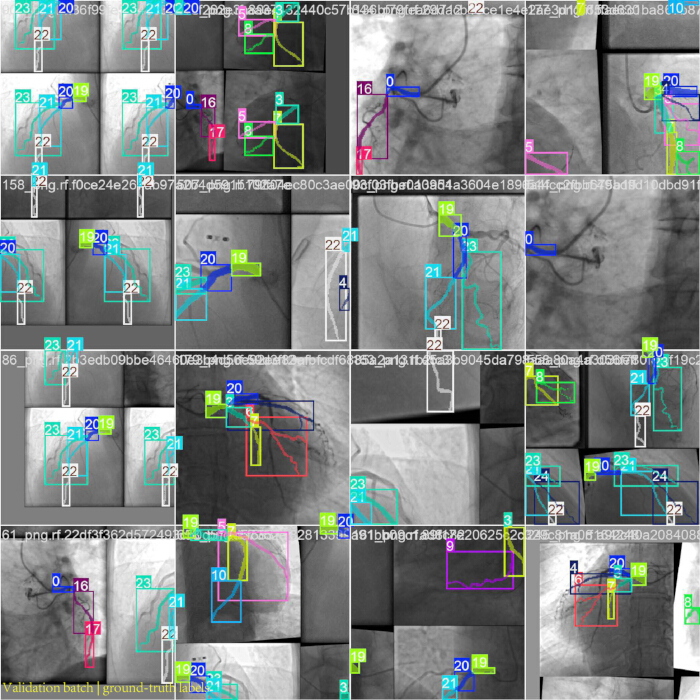
Figure 4: Annotated validation-batch samples from the YOLO26-seg run on the ARCADE dataset. The on-figure title reads “Validation batch | ground-truth labels.” The 4 × 4 mosaic is the Ultralytics validation-batch view from the same run. Colored rectangles are ground-truth bounding boxes, colored contours are ground-truth segmentation masks, and the integers are 0-based class indices for the 25 ARCADE labels, rather than the segment names used in Figure 3. Several tiles show overlapping boxes or small, low-contrast segments. The mosaic does not overlay predictions from YOLO26-seg or from the other models and is not used to rank architectures. Please click here to view a larger version of this figure.

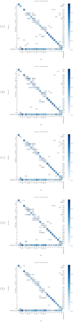
Figure 5: Normalized confusion matrices for YOLO segmentation variants on the ARCADE validation set. (A) YOLOv8-seg. (B) YOLOv9c-seg. (C) YOLO11-seg. (D) YOLO12-seg. (E) YOLO26-seg. Each matrix shows predicted versus true class assignments, with values normalized by the true-class counts. Please click here to view a larger version of this figure.

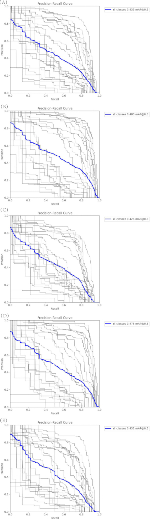
Figure 6: Precision–recall curves for box and mask predictions on the ARCADE validation set. (A) Box PR curve for YOLOv9c-seg. (B) Mask PR curve for YOLOv9c-seg. (C) Box PR curve for YOLOv8-seg. (D) Mask PR curve for YOLOv8-seg. (E) Box PR curve for YOLO11-seg. Each panel reports per-class and all-class performance on the validation set. Please click here to view a larger version of this figure.

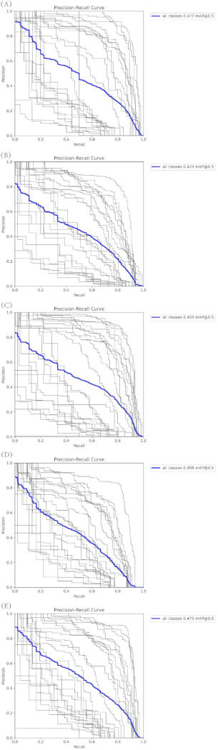
Figure 7: Precision–recall curves for box and mask predictions on the ARCADE validation set (continued). (A) Mask PR curve for YOLO11-seg. (B) Box PR curve for YOLO12-seg. (C) Mask PR curve for YOLO12-seg. (D) Box PR curve for YOLO26-seg. (E) Mask PR curve for YOLO26-seg. Each panel reports per-class and all-class performance. Please click here to view a larger version of this figure.

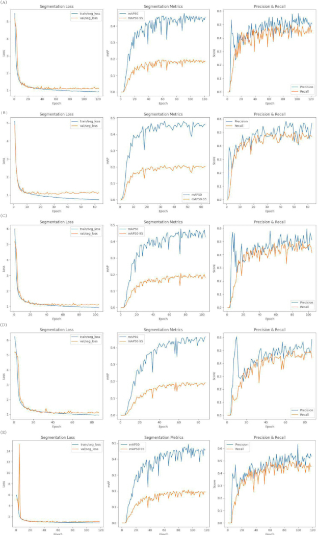
Figure 8: Custom training visualizations for YOLO segmentation variants on the ARCADE dataset. (A) YOLOv8-seg, 121 epochs. (B) YOLOv9c-seg, 63 epochs. (C) YOLO11-seg, 104 epochs. (D) YOLO12-seg, 87 epochs. (E) YOLO26-seg, 118 epochs. In each lettered block, the left panel shows training and validation segmentation loss, the middle panel shows mask mAP@50 and mAP@50–95, and the right panel shows precision and recall. Please click here to view a larger version of this figure.

Table 1: Inference timing and training characteristics of the YOLO segmentation models. Inference time and approximate FPS were measured on the reported A100/FP32 setup and are not end-to-end clinical latency. Training duration, model size, and peak GPU memory are reported as observed training characteristics; batch size, optimizer, and epoch settings are not included in this table. Please click here to download this file.

Table 2: Post hoc test-split evaluation of the original best checkpoints on the Roboflow v1 test split (n = 150 images, 795 instances). Values are all-class box and mask precision, recall, mAP@50, and mAP@50–95 transcribed from the supplied Ultralytics 8.4.157 log recorded on a Tesla T4. Please click here to download this file.

Table 3: Validation performance of five YOLO segmentation models on the ARCADE validation set (n = 299). Values are bounding-box and mask precision, recall, mAP@50, and mAP@50–95. Please click here to download this file.

Table 4: Per-class mask mAP@50 and mAP@50–95 on the 25 ARCADE anatomical classes. Major segments (classes 1–8 and 11) reach mask mAP@50 above 0.65 for most models. Class 9 does not meet this threshold (mask mAP@50 approximately 0.40–0.44). Rare variants and small branches (classes 10, 10a, 12, 12a, 12b, 14, 14a, 14b, 15, 16a, 16b, and 16c) are substantially lower, and several fall below 0.30 mask mAP@50. Please click here to download this file.

Table 5: Architectural summary of YOLO-segmentation variants evaluated in this study. Total number of layers, parameter count, GFLOPs, and model size (MB) for YOLOv8-seg (86 layers, 3,262,939 parameters, 11.4 GFLOPs, 6.8 MB), YOLOv9c-seg (169 layers, 27,643,803 parameters, 147.7 GFLOPs, 56.3 MB), YOLO11-seg (114 layers, 2,839,443 parameters, 9.6 GFLOPs, 6.0 MB), YOLO12-seg (172 layers, 2,814,019 parameters, 9.6 GFLOPs, 6.1 MB), and YOLO26-seg (139 layers, 2,693,759 parameters, 9.0 GFLOPs, 6.6 MB). Please click here to download this file.

Обсуждение

This study provides a methodological benchmark of five YOLO-segmentation models on the public ARCADE dataset. The validation comparison identified YOLOv9c-seg as the highest observed validation mask mAP@50–95 model, while the post hoc test log showed YOLO11-seg with the highest observed test mask mAP@50–95. The test results are descriptive single-seed results, and the A100 throughput measurements indicate model-level computational performance rather than clinical readiness.

Major anatomical segments were consistently well-segmented across architectures, whereas rare variants and small branches remained challenging, primarily due to severe class imbalance and low-contrast features inherent to X-ray angiography. These performance patterns were consistent with the per-class analysis and confusion matrices presented in the results section.

The dataset-preparation stage used the Roboflow v1 export settings (Auto-Orient and stretch to 640 × 640 pixels). Training-time transformations were applied by the Ultralytics pipeline and were not applied to validation or test images. Transfer learning used explicit pretrained segmentation checkpoints. Batch size was adjusted when GPU memory was insufficient, and early stopping was used with a patience of 30 with validation-fitness checkpoint selection. Common troubleshooting issues and solutions are as described above.

This study has several limitations. All reported scores come from a single deterministic seed (seed 0). Repeated-seed variability and confidence intervals are not available, so differences between models—including the small gaps in test mask mAP@50–95—are descriptive single-seed observations and are not statistically significant comparisons. The Roboflow v1 release provides an image-level 3,138/299/150 train/validation/test split, but the available materials do not certify patient-level disjointness or exclude frames from the same patient across subsets. Model selection used the validation subset, so validation-set optimism remains possible. The test results were obtained by post hoc evaluation of the saved checkpoints and should not be interpreted as independent patient-level external validation. The five architectures are not size-matched because YOLOv9c-seg is much larger, and the effective batch size differed when memory required reduction. Box and mask precision, recall, mAP@50, and mAP@50–95 are reported; Dice, IoU/mIoU, sensitivity, specificity, and boundary or Hausdorff-type metrics could not be derived from the stored outputs in this revision. Direct numerical equivalence with studies that report those overlap and boundary metrics is therefore not implied. Timing was measured on specified GPUs and is not full clinical workflow latency. No same-protocol U-Net or nnU-Net baseline was completed, and no clinical outcome or prospective workflow benefit was measured.

Future work should create a patient-level split manifest with explicit overlap checks, repeat training across multiple seeds, and report confidence intervals or paired statistical comparisons. A same-dataset U-Net or nnU-Net baseline should use the same resolution, split, hardware, and timing protocol. Subsequent evaluation should add Dice, IoU/mIoU, sensitivity, specificity, and boundary or Hausdorff-type metrics when full prediction masks can be retained. To address the severe class imbalance documented in Figure 1A and Table 4, training should add class-aware or repeat-factor sampling of rare segments (10, 10a, 12, 12a, 12b, 14, 14a, 14b, 15, 16a, 16b, and 16c), class-weighted or focal losses, and anatomy-constrained copy-paste synthesis of minority branches, together with targeted collection of those labels. End-to-end timing should include preprocessing, transfer, mask decoding, post-processing, and display on representative clinical hardware. Cross-dataset validation and prospective workflow studies are required before claims about clinical utility or deployment can be made.

Материалы

Список материалов, использованных в этой статье

Имя	Компания	Каталожный номер	Комментарии
YOLOv8-seg	Ultralytics	(https://github.com/ultralytics/ultralytics)
YOLOv9c-seg	WongKinYiu	(https://github.com/WongKinYiu/yolov9)
YOLO11-seg	Ultralytics	(https://github.com/ultralytics/ultralytics)
YOLO12-seg	Ultralytics	(https://github.com/ultralytics/ultralytics)
YOLO26-seg	Ultralytics	(https://github.com/ultralytics/ultralytics)
PyTorch (v2.10.0)	PyTorch Foundation	(https://pytorch.org/)
Python (v3.12.13)	Python Software Foundation	(https://www.python.org/)
CUDA (v12.8)	NVIDIA	(https://developer.nvidia.com/cuda-toolkit)
Ultralytics (v8.4.51)	Ultralytics	(https://github.com/ultralytics/ultralytics)
Ultralytics (v8.4.157)	Ultralytics	(https://github.com/ultralytics/ultralytics)
Albumentations	Albumentations Team	(https://albumentations.ai/)
NumPy	NumPy Community	(https://numpy.org/)
Matplotlib	Matplotlib Community	(https://matplotlib.org/)
Pandas	Pandas Community	(https://pandas.pydata.org/)
ARCADE Dataset	ARCADE Challenge	(https://www.arcade-challenge.com/)
Google Colab Pro	Google	(https://colab.research.google.com/)
NVIDIA A100-SXM4-40GB GPU	NVIDIA	(https://www.nvidia.com/)
Ubuntu (Linux)	Canonical	(https://ubuntu.com/)
VGG Image Annotator (VIA v3.0.11)	University of Oxford	(https://www.robots.ox.ac.uk/~vgg/software/via/)
Roboflow	Roboflow	(https://roboflow.com/)
NVIDIA Tesla T4 GPU	NVIDIA	(https://www.nvidia.com/)