Quantifying Polarity and Dynamics of a Secretion System Component in Legionella pneumophila

Abstract

Source: Chetrit, D., et al. Applying Live Cell Imaging and Cryo-Electron Tomography to Resolve Spatiotemporal Features of the Legionella pneumophila Dot/Icm Secretion System. J. Vis. Exp. (2020)

This video demonstrates the use of live-cell fluorescence imaging to quantify the polarity and dynamics of secretion system components in Legionella pneumophila, enabling analysis of spatial recruitment and cytosolic redistribution critical for understanding bacterial pathogenesis

Protocol

1. Quantification of Polar Localization and Dynamics of Dot/Icm Components

NOTE: The following steps are designed for images with 0.129 µm per pixel that were acquired with 2 x 2 binning.

1. Quantification of polarity for sfGFP (superfolder green fluorescent protein) fusion proteins (Figure 1)
   1. Adjust the image contrast so the bacteria are clearly visible. Use the region tool to place a 0.25 x 1.3 µm² rectangle starting at the pole and extending into the cytoplasm. The rectangle must remain precisely within the bacterial borders.
   2. Mark at least 200 bacteria and use the

Results

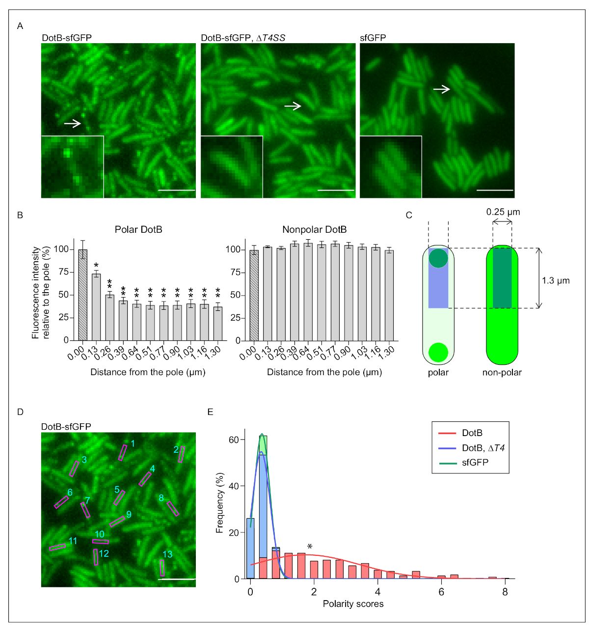
Figure 1: Quantification of polar localization of Dot/Icm system subunits. (A

Materials

List of materials used in this article

Name	Company	Catalog Number	Comments
100x Plan Apo objective (1.4 NA)	Nikon
CoolSNAP EZ 20 MHz digital monochrome camera	Photometrics
Microscope cover slides 22x22 mm	Fisher Scientific	12-542B
Microscope cover slides 24x50 mm	Fisher Scientific	12-545K
Microscope slides 25x75x1 mm	Globe Scientific	1380
SlideBook 6.0	Intelligent Imaging Innovations
Spectra X light engine	Lumencor