Two-Photon Microscopy for Studying Microglial Process Attraction Toward a Compound in a Mouse Brain Slice

Abstract

Source: Etienne, F. et al. Two-photon Imaging of Microglial Processes' Attraction Toward ATP or Serotonin in Acute Brain Slices. J. Vis. Exp. (2019)

This video demonstrates the use of two-photon microscopy to study the attraction of microglial processes toward an injected compound in brain slices. It provides an overview of preparing mouse brain slices, injecting a chemoattractant test compound, and imaging fluorescently labeled microglia to visualize their responses.

Protocol

All procedures involving animal samples have been reviewed and approved by the appropriate animal ethical review committee.

1. Two-photon Microscopy

1. Parameters setting
   1. Switch on the multiphoton system (hybrid detectors, laser, scanner, electro-optic modulator, microscope).
   2. Tune the laser at 920 nm, check that the laser is mode-locked, and set the power at 5% - 15% and the gain at 10%. This corresponds to a power of 3 - 5 mW under the objective. Ensure that the nondescanned detectors are engaged and that the appropriate emission and excitation filters installed.
   3. Set parameters of the imaging software to the following values: for the frame size, 1024 x 1024 pixels corresponding to an area of 295.07 x 295.07 µm; for the zoom, 2. If the signal is very noisy, apply a line average of 2. For the pixel dynamics, set the imaging software at 12 bits or more.
      NOTE: Images with a higher bit value allow researchers to distinguish smaller differences in fluorescence intensity than images with a lower bit value: a change of one gray value in an 8-bit image would correspond to a change of 16 gray values in a 12-bit and of 256 gray values in a 16-bit image. Therefore, higher-bit images are more appropriate for quantitative analysis, but as their size increases with bit depth, storage capacity, and computing power can become limiting.
   4. Select the scan mode XYZT with a Z-interval range at 2 µm and a T-interval of 2 min.
      NOTE: The x,y and z resolution are determined by the Nyquist sampling theorem. A Z-step size of around 0.8 would be optimal to resolve microglia processes (with a diameter of <1 µm), but the optical resolution of multiphoton microscopy is limiting (at 920 nm with a 0.95 NA objective, the axial resolution is around 1 µm). On top of that physical barrier, in a live-imaging experiment, the sensitivity or signal-to-noise ratio, the resolution, the speed, and the total observation time matter. Taking into account all these parameters, a z-step of 2 µm, an image size of 1024 x 1024 pixels, and a high-speed acquisition using a resonant scanner coupled to HyD detectors (it takes around 15 s to acquire 50 z-plans) were selected here. The frequency of acquisitions is one XYZT series every 2 min, and the total duration is 30 min. If the set-up is not fast or sensitive enough, it is possible to reduce the lateral resolution (down to 512 x 512) or the number of z-slices (by imaging exclusively in the z-depth which exhibits the strongest fluorescence [i.e., not the deepest z-slices where fluorescence is faint]), or to decrease the speed of the scanner. The axial resolution can also be decreased by increasing the z-step up to 3 µm, but as this may impact the quantification, all experiments to be compared should be performed with the same z-step.
      NOTE: It is possible to perform similar experiments on slices from CX3CR1creER-YFP mice, a mouse line used to induce genetic deletion in microglia only and in which microglia constitutively express yellow fluorescent protein (YFP). However, the expression level of YFP is very low compared to green fluorescent protein (GFP) in CX3CR1^GFP/+ mice; thus, imaging is possible but challenging and requires the optimization of the acquisition parameters. It is recommended to adjust them as follows.
   5. Tune the laser at 970 nm (which is better adapted to YFP excitation than 920 nm), the power at 50%, and the gain at 50%, which corresponds to a laser power under the objective of 5 - 6 mW.
   6. Set a line average of 4 (or more) to improve the signal-to-noise ratio.
2. Positioning of the slice and of the glass micropipette, and the local application of the compound
   1. Connect the peristaltic pump to the recording chamber, 30 min before starting the recording. After cleaning the whole perfusion system with 50 mL of ultrapure water, start the perfusion of the recording chamber with aCSF (50 mL) contained in a glass beaker under constant carbogenation. Throughout the experiment, keep the circulating aCSF to 32 °C with an inline microheater or a Peltier heater.
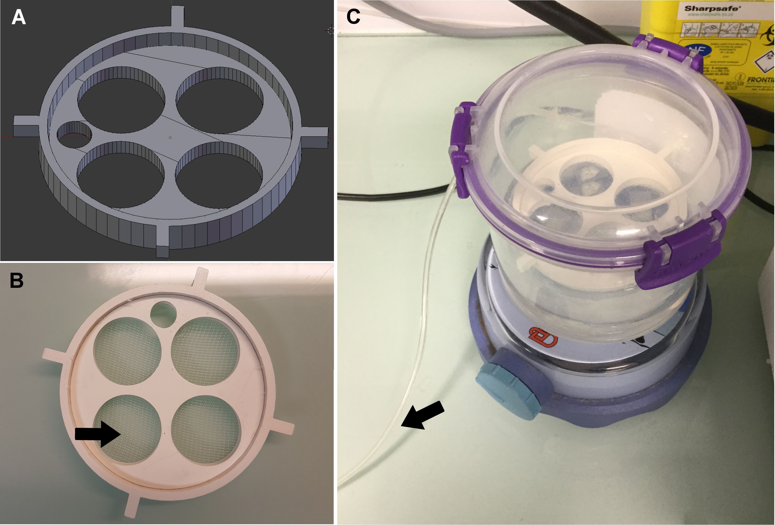
      NOTE: A specific perfusion chamber with top and bottom perfusion is designed to optimize the oxygenation on both sides of the slice. The perfusion chamber is composed of two perfectly fitting parts, with a polyamide mesh stretched between them (Figure 1A,B). Compared with other types of chambers, where the slice is directly laying on a glass coverslip, this chamber reduces neuronal death in the bottom part of the slice, improves viability, and reduces the slice movements induced by its swelling.
   2. With a wide-mouth disposable transfer pipette, transfer the brain slice to be imaged to the aCSF beaker to remove the lens paper, let it sink (as a proof that no air bubble is attached), and transfer it to the recording (perfusion) chamber.
   3. Position a slice holder (a hairpin made of platinum with the two branches joined by parallel nylon threads) on the slice to minimize slice movement due to the perfusion flow.
   4. Use the bright-field illumination to target the brain region of interest (exposure time: 50 to 80 ms) using a low magnification objective (5X or 10X). Switch to the higher magnification (25x with a 0.35x lens) water immersion objective and adjust the position.
      NOTE: Avoid to image fields close to the slice holder’s nylon threads as they can block the light and locally deform the slice. Make sure that the area of interest is flat. If necessary, remove the slice holder in order to reposition the slice and/or the slice holder.
   5. Use the fluorescence illumination to locate fluorescent microglial cells to be imaged in the field (exposure time: 250 - 500 ms).
      NOTE: This step allows researchers to check the presence of cells in the region of interest and their fluorescence intensity, and to control for the amount of cellular debris.
   6. Backfill the pipette with 10 µL of aCSF with ATP, 5-HT, or the drug of interest at its final concentration. Point the tip downward and gently shake the drug-filled pipette to remove any air bubbles trapped in the tip.
      NOTE: If the solution to be injected tends to form bubbles, consider using borosilicate pipettes with an internal filament. Leakage of ATP out of the pipette can attract microglial processes even before the injection (if this occurs, it will be visible at the analysis step). Although this should be moderate with the ATP concentration used (500 µmol·L^-1), if it is an issue, consider prefilling the micropipette with 2 mL of aCSF prior to adding the ATP (or other compound) solution at step 1.2.6.
   7. Mount the filled pipette in a pipette holder, connected with transparent tubing to a 5 mL syringe, with a plunger positioned at the 5 mL position. The pipette holder itself is mounted onto a three-axis micromanipulator.
   8. Under bright-field illumination, use the micromanipulator to position the pipette in the center of the field. For a reproducible and optimal centering, display and use the rulers on the image.
   9. Lower the pipette gently toward the slice, controlling and adjusting the objective at the same time until the pipette tip lightly touches the surface of the slice. Stopping the descent of the pipette as soon as it is visible that the slice has been touched allows the pipette tip to penetrate 80 - 100 µm of the surface of the slice (see Figure 2B).
   10. Tune the laser (see the parameters above) and switch the microscope to the multiphoton mode. Make sure that the chamber is screened from any light source (e.g., a computer screen). Switch on the nondescanned detectors and set the gain. Use a lookup table (LUT) with a color-coded upper limit to avoid saturating the pixels in the image.
   11. Determine the thickness of the slice to be imaged (i.e., the upper and lower z-positions where fluorescence is detectable [usually between 220 and 290 µm in total]).
       NOTE: At the surface of the slice, there is an increased density of processes and possibly of microglia, often with an unusual morphology, in comparison with the inside of the slice. This accumulation will be more striking with time (i.e., more visible in the last than in the first brain slice to be imaged). Therefore, the z-planes in the first ~30 µm should not be used for the analysis and can even be skipped for the acquisition.
   12. Start recording for a total duration of 30 min (or more if desired) and after a 5 min baseline, locally apply the compound to be tested (without interrupting the imaging). To do this, slowly press the plunger of the syringe connected to the micropipette, from the 5 mL to the 1 mL position (in about 5 s). Resistance when pressing the plunger must be felt immediately. If not, the tip might be broken.
       NOTE: For a trained experimenter, the injections with this method are reproducible, but alternatively to the manual manipulation of a syringe, the pipette could be linked to an automated pressure ejection system to allow better control of the volume delivered. The injection creates a physical distortion of the slice at the site of the injection. This distortion is visible a posteriori in the first two or three images after the injection but should not be visible on the fourth image (i.e., 8 min after the injection). If it persists, consider changing the parameters for the pipette preparation.
   13. At the end of the acquisition (30 min), discard the micropipette and remove the slice.
   14. Prior to starting to image a new slice, make the 2D movie (section 2.1) in order to check that microglia have a normal morphology and are moving and, thus, that the slices are healthy.

2. Analysis of the Attraction of Microglial Processes

1. 2D projection and drift correction
   1. Open the file (.LIF) with Fiji.
   2. If necessary, make a substack (Image/Stacks/Tools/Make Substack) with only the z-planes of interest. For example, exclude the z-planes corresponding to the surface of the slice if they have been acquired but are not to be used for the analysis (see the NOTE after step 1.2.11) and the deepest z-planes with no fluorescence. The final stack generally contains 90 - 110 z-slices (180 - 220 µm).
   3. Launch the Z project function (Image/Stacks/Z Project") and select the Max Intensity projection type to make the projections of the z-stack acquired at each time point.
   4. Launch the MultiStackReg plugin (Plugin/Registration/MultiStackReg), selecting Action 1: Align and Transformation: Rigid Body to correct slight drifts that may have occurred during the acquisition. Save this 2D movie as a new file (.tiff).
2. Data processing
   1. Open this new file with Icy.
   2. Draw a circular R1 region of interest (ROI) of 35 µm in diameter, centered on the injection site (identified notably by the shadow of the pipette and the distortion created at the time of injection).
   3. Use the plugin ROI intensity evolution and measure the mean intensity over time in R1.
   4. Save the results to an .XLS file.
3. Quantification and representation of the results
   1. To quantify the microglial response over time, determine at each time point.
      Then, the results can be represented as a kinetic of the microglial response, or at a specific time point (see Figure 3).

Results

Figure 1: Interface chamber details. (A) Outline for the 3D printing of the slice holder. The external diameter of the holder is 7 cm. (B) Interface slice holder with...

Materials

List of materials used in this article

Name	Company	Catalog Number	Comments
for slice imaging
× 25 0.95 NA water-immersion objective	Leica Microsystems (Germany)	HCX Irapo
2-photon MP5 upright microscope with resonant scanners (8 kHz) and two HyD Hybrid detectors	Leica Microsystems (Germany)
Antlia-3C Digital Peristaltic pump	DD Biolab	178961	For 2-photon chamber perfusion with aCSF
Carbogen 5% carbon dioxide/95% oxygen	Air Liquide France Industrie	I1501L50R2A001
Chameleon Ultra2 Ti:sapphire laser	Coherent (Germany)
Disposable transfer pipettes , wide mouth	ThermoFischer scientific	for example : 232-11	5.8ml with fin tip, but we cut it (approx 7cm) to have a 4 mm diameter mouth
Emission filter SP680	Leica Microsystems (Germany)
Fluorescent cube containing a 525/50 emission filter and a 560 dichroic filter (for fluorescence collection)	Leica Microsystems (Germany)
Glass beaker with 50 mL of ACSF to maintain constant perfusion of the slice
Heating system	Warner Instrument Corporation	Automatic Heater Controller TC-324B	to maintain perfusion solution at 32°C
Perfusion chamber			home-made, the file for 3D printing is provided in Supplemental Material
Slice holder ("harp")			home made : hairpin made of platinum with the two branches joined by parallel nylon threads
For slice stimulation
Adenosine 5′-triphosphate disodium salt hydrate (ATP)	Sigma	A-26209	to be prepared ex-temporaneously : 1mg/ml (3mM) stock solution prepared the day of the experiment, kept at 4°C (a few hours) and diluted just before use
Fluorescein (optional)	Sigma	F-6377	use at 1 µM final
Micromanipulator	Luigs and Neumann	SM7	connected to the micropipette holde
Micropipette holder			same as for eletrophysiology
Serotonin hydrochloride	Sigma	H-9523	aliquots of 50mM stock solution in H20 kept at -20°C. 500µM solution prepared the day of the experiment.
Syringe 5mL (without needle)	Terumo medical products	SS+05S1
Transparent tubing	Fischer Scientific	11750105	Saint Gobain Performance Plastics™ Tygon™ E-3603 Non-DEHP Tubing
For image analysis
Fiji		https://fiji.sc
Icy	Institut Pasteur	http://icy.bioimageanalysis.org
Mice
CX3CR1-GFP mice	Jung et al, 2000		male or females, P3 to 2 months-old ; we have backcrossed these mice on 129sv background.
CX3CR1creER-YFP mice	Parkhurst et al 2013		male or females, P3 to 2 months-old ; we have backcrossed these mice on 129sv background.