Two-Color Stimulated Raman Scattering Imaging of Mouse Brain Tissue

Abstract

Source: Espinoza, R., et al. Real-Time, Two-Color Stimulated Raman Scattering Imaging of Mouse Brain for Tissue Diagnosis. J. Vis. Exp. (2022).

The video demonstrates two-color stimulated Raman scattering (SRS) imaging of mouse brain tissue sections. Two synchronized laser beams are directed onto the tissue section to excite molecular vibrations, resulting in a relative intensity change in the beams. Lipids and proteins in the tissue are detected using distinct frequency pairs of the laser beams. The resulting signals are then assigned separate colors, creating a two-color image that helps identify the proteins and lipids in the tissue.

Protocol

All procedures involving animal samples have been reviewed and approved by the appropriate animal ethical review committee.

1. SRS signal detection

1. Electrooptical modulation (EOM)
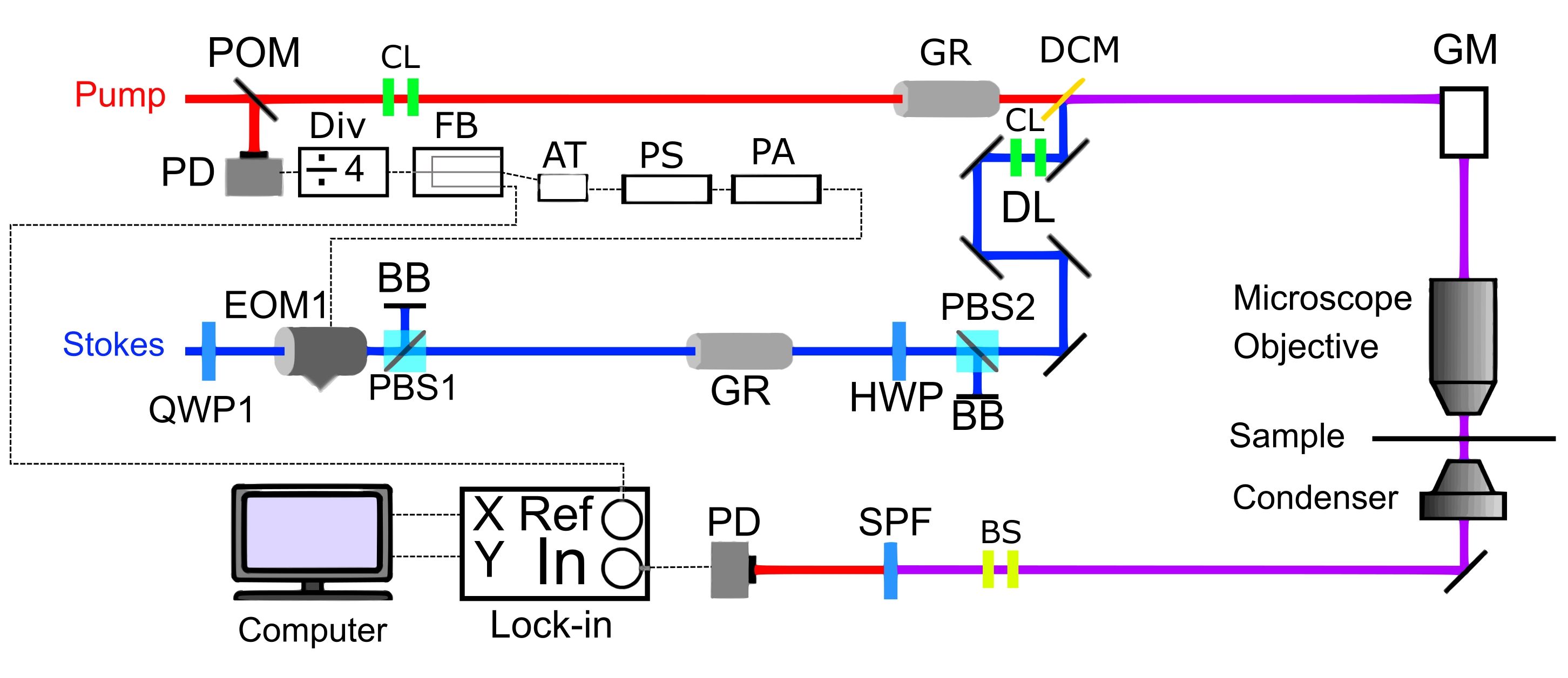
   NOTE: EOM of 20 MHz is used to modulate the Stokes amplitude. As discussed later, the EOM is derived from the 80 MHz laser pulse train, which is required for orthogonal modulation. Other modulation frequencies can be used if only single-color or hyperspectral SRS is performed. In that case, synchronization of modulation frequency to laser frequency is unnecessary. A frequency generator with a radiofrequency (RF) power amplifier can be used to drive EOM. As a result, steps 1.1.1-1.1.4 can be skipped.
   1. Place a beam sampler in the Stokes beam path to pick up 10% of the beam and send it to a fast photodiode to detect the 80 MHz pulse train.
      NOTE: The photodiode signal is sent to a frequency divider to generate a 20 MHz TTL output. This output is further sent into a fanout buffer to replicate the output into four identical 20 MHz outputs. One of the outputs is used to trigger the oscilloscope.
   2. Take one of the outputs of the fanout buffer and filter it with a bandpass filter to get a 20 MHz sinusoidal wave. Use an RF attenuator to adjust the output peak-to-peak voltage to ~500 mV.
   3. Send the resulting output to a phase shifter, which allows fine adjustment of the RF phase with a voltage source. Send this output to an RF power amplifier and connect the output of the amplifier to EOM.
   4. Unblock the Stokes beam and optimize the modulation depth of EOM1 by placing a photodiode in the beam path. Adjust the EOM voltage and quarter-wave plate until the modulation depth (valley to peak ratio) appears satisfactory.
      NOTE: At 20 MHz modulation (1/4 of the laser repetition rate), two pulses are expected every 50 ns.
2. Temporal overlap
   NOTE: Temporal overlap of the pump and Stokes is achieved by delaying one of the two laser pulse trains with a retroreflector mounted onto a delay stage (Figure 1 shows the Stokes being delayed). Coarse overlap is monitored with the oscilloscope, and fine overlap is monitored by the SRS signal. Fine temporal overlap can also be achieved with an autocorrelator if available.
   1. Place a photodiode after the dichroic mirror to detect the laser beam. Block the Stokes beam first. Zoom in on one of the pump pulse peaks on the oscilloscope. Place a vertical cursor to mark the temporal position of this peak with the oscilloscope.
   2. Block the pump beam and unblock the Stokes beam. Translate the delay stage to temporally match the peak position on the oscilloscope to the marked position in the previous step. See Figure 2 for a display of the temporal overlap of two beams.
      1. (OPTIONAL) If the translation of the delay stage is insufficient to temporally match the two beams, then move the delay stage to the middle of its movement range.
      2. Calculate the delay distance required to match the two beams by taking the temporal difference between the two beams and multiplying the difference by the speed of light to find the amount of distance needed to match the two beams temporally.
      3. Elongate the beam path of the faster beam or shorten the beam path of the slower beam to roughly match the temporal delay accordingly.
   3. Prepare a microscope slide sample with dimethyl sulfoxide (DMSO) and double-sided tape as a spacer to hold the sample between the slide and a coverslip.
   4. Place the sample on the microscope with the coverslip side facing the microscope objective. Change the microscope to brightfield illumination and observe the sample from the eyepiece. Find the focus of the sample by first finding the focus at both the top and bottom layer of air bubbles at the glass-tape interface, and then move the focus to be in between the two layers of tape.
      NOTE: Ensure the laser beams are blocked before looking into the eyepiece.
   5. Set the tunable beam output to 798 nm. Based on the optical throughput of the condenser, adjust the optical power to be ~40 mW each for the pump and Stokes beams at the objective focus.
   6. Open ScanImage in MATLAB (or other scanning software that controls the microscope) and click on the button labeled FOCUS to start scanning.
      NOTE: The laser beams will be raster-scanned through the sample to generate an image. The low-frequency signal output from the photodiode (<100 kHz) is directly sent into channel 1 of the data acquisition card (referred to as the DC channel). The high-frequency output (>100 kHz) from the photodiode is sent into the lock-in amplifier, and the X-output of the lock-in amplifier signal is sent into channel 2 of the data acquisition card (referred to as the AC channel).
   7. Adjust the steering mirror before the galvo scanner to center the DC signal on the channel 1 display. Move the motorized delay stage and closely observe the lock-in output shown on the channel 2 (i.e., AC channel) display.
      NOTE: When the pump and Stokes coincide in time, a signal will show up on the AC channel. It is helpful to adjust the color scale of the AC channel to display the small intensity change.
   8. Maximize the AC signal intensity by finely adjusting the time delay. Adjust the dichroic mirror to center the SRS signal on the AC channel (while keeping the DC channel centered). Adjust the phase of the lock-in amplifier to maximize the signal. See Figure 3 for a satisfactory signal.

3. Spectral resolution optimization

NOTE: The pump and Stokes beams reaching the sample should have the same amount of group delay dispersion (GDD) to maximize spectral resolution. The dispersion depends heavily on the experimental setup. The experimental setup described here utilizes femtosecond pulses at 1,040 nm and 800 nm as Stokes and pump, respectively. Dense flint glass rods (H-ZF52A) are used as the pulse-stretching medium.

1. Insert 48 cm of a highly dispersive glass rod (H-ZF52A or equivalent dense flint glass) into the 800 nm beam path. Estimate the GDD using Eq (1):

   

   NOTE: GVD of various glass materials at different wavelengths can be found from the refractive index database resource. For example, H-ZF52A has a GVD of 220.40 fs²/mm at 800 nm. The total GDD is 105792 fs².

2. Calculate how many cm of the dispersive glass rod is required to add to the 1,040 nm beam path to match the GDD of the pump. Insert the appropriate length of dispersive glass rods into the 1,040 nm beam path to roughly match the GDD of the 800 nm beam. Note that the addition of glass rods will change the temporal overlap of the two beams, and adjustment of the delay may be necessary.
3. Calibration of spectral resolution
   1. Make a microscope slide sample with DMSO. Place the slide onto the microscope and check the power of the beams coming out of the microscope condenser. Adjust the power accordingly to have ~40 mW each at the sample focus.
   2. Open ScanImage from MATLAB. Find the maximal SRS signal by scanning through the delay stage, which corresponds to the 2,913 cm^-1 Raman peak of DMSO. Estimate the stage position based on the previous stage position with the increased optical path length due to the insertion of rods. Realign the beam spatial overlap because of the small deviation of the beam when glass rods are added.
   3. Save a hyperspectral SRS scan by sequentially taking a series of SRS images while moving the motorized stage.
      NOTE: The delay scan range covers two Raman peaks, corresponding to the 2,913 cm^-1 and 2,994 cm^-1 Raman peaks of DMSO, respectively. These two transitions are observed when utilizing an 800 nm pump and a 1,040 nm Stokes laser.
   4. Plot out the SRS spectra of the DMSO solution using either ImageJ or MATLAB. Fit the large DMSO 2,913 cm^-1 peak to a Gaussian or Lorentzian function in MATLAB to calculate the Full Width at Half Maximum (FWHM) of the peak.
      NOTE: Representative results are shown in Figure 4. If only one broad peak is present, that means either the spectral resolution is too poor to distinguish the two peaks and more glass rods are required, or the scanned range was too small to detect the second peak. Typically, an acceptable spectral resolution DMSO is ~20-25 cm^-1 when a glass rod length of >60 cm is used. A lower resolution is often used for tissue imaging to trade for higher signals with shorter pulses.
4. (OPTIONAL) Use an autocorrelator or a FROG (Frequency-Resolved Optical Gating) to determine the pulse duration of each arm to calculate exactly the amount of GDD and the length of rods needed to match the GDD between the pump and the Stokes.
5. Repeat steps 3.3.2-3.3.4 for different rod lengths on the Stokes beam to find the optimal spectral resolution, which means the best GDD match has been found experimentally. Use multiple sets of glass rods differing in length to achieve optimal spectral resolution.

4. Signal-to-noise (SNR) characterization

1. Ensure that step 4.2 is performed after complete spatial and temporal alignment.
2. Acquire an SRS image corresponding to the 2,913 cm^-1 Raman peak of DMSO. Open the image in ImageJ and select a small area in the center of the frame. Use the measure function to calculate the mean and standard deviation of values in the selected area.

3. Divide the mean value of the selected area by the standard deviation to find the SNR value, as in Eq (2).

   

   NOTE: A good SNR for the system (with a lock-in time constant of 4 μs) using DMSO at 40 mw/40 mw at focus for both arms is >800. Lower concentrations of DMSO or lower power can be used for a more accurate estimation of the SNR if the data acquisition card has a limited bit depth.

4. If the SNR is too low, realign the laser pulses to optimize spatial overlap, temporal overlap, beam size/collimation matching, and/or dispersion matching. For an objective with an aberration correction collar, optimize the signal by adjusting the correction collar.

5. Frequency axis calibration

NOTE: This step is performed to relate the delay stage position to the scanned Raman transition. Careful selection of solvents is required to generate an appropriate "Raman Ruler." DMSO is an effective solvent for CH bonds as it has two sharp Raman peaks at 2,913 cm^-1 and 2,994 cm^-1.

1. Save a hyperspectral scan with the delay-stage range covering the 2,913 cm^-1 and 2,994 cm^-1 Raman peaks of DMSO. Save the stage positions corresponding to the hyperspectral dataset.
   NOTE: The global maximum peak of the spectrum corresponds to the DMSO 2,913 cm^-1 Raman shift and the second maximum peak corresponds to the DMSO 2,994 cm^-1 Raman shift.
2. Perform linear regression for the stage positions and Raman shifts at 2,913 cm^-1 and 2,994 cm^-1. Using the linear regression equation relating the stage position to the Raman shift, convert the delay positions to the corresponding Raman frequencies.

6. Orthogonal modulation and two-color imaging

NOTE: The orthogonal modulation step is only necessary when real-time two-color imaging is needed. The schematic of this scheme is shown in Figure 5. The orthogonal modulation uses a pair of EOMs driven at a quarter of the laser frequency (20 MHz for an 80 MHz laser) with a 90° phase shift between the two. This orthogonal modulation step can be skipped for single-color SRS imaging or hyperspectral SRS imaging.

1. EOM1 modulation
   1. Install a polarizing beam splitter (PBS2), a quarter-wave plate (QWP2), and a second EOM (EOM2) into the Stokes beam path after the first EOM. Unplug the signal input to EOM2. Plug in the signal input to EOM1 and turn it on.
   2. Modulate the Stokes beam (fixed at 1,040 nm) at 20 MHz (f₀/4) by sending the beam through the first EOM. Adjust the tilt and position of EOM1 to ensure that the beam is hitting straight and centered through the EOM crystal.
   3. Monitor the modulation depth by observing both polarizations coming out of PBS1 with two photodiodes and displaying the modulation on an oscilloscope.
   4. Adjust the QWP1, EOM1 voltage, and phase of the 20 MHz input (using a phase shifter) to optimize the modulation depth of the transmitted beam to be close to 100%. See Figure 2B for an illustration of good modulation depth.
2. EOM2 modulation
   1. Unplug EOM1 and plug in EOM2.
   2. Send in the high voltage output of the second amplifier at 20 MHz to EOM2. Adjust the tilt and position of EOM2 to ensure that the beam is hitting straight and centered through the EOM crystal.
   3. Once again, monitor the modulation depth by looking at both polarizations coming out of PBS2 with an oscilloscope. Adjust the QWP2, EOM2 voltage, and the phase shifter as needed to achieve close to 100% modulation for both polarizations.
   4. Ensure that the pulse train modulation has a 90° phase shift from the first modulation.
      NOTE: If the two pump pulse trains are not 90° orthogonal, crosstalk between the two channels will be a problem.
   5. Test the orthogonality of the modulation by turning on and plugging in both EOM1 and EOM2. Monitor both polarizations being split by PBS2 with an oscilloscope. Reoptimize EOM1 and EOM2 individually if the pulse train after the second PBS does not resemble Figure 2C.
   6. Install a 20 mm birefringent quartz crystal (BRC) and half-wave plate (HWP) downstream of EOM2. Plug in both EOMs at once and monitor the pulse train such that it resembles Figure 2D.
      NOTE: For the chirp used in this experiment, 20 mm BRC induces a time delay that corresponds to an 80 cm^-1 Raman shift. A different BRC length may be needed if a different chirp is used.
3. Calibration
   1. Calibrate the system using DMSO by detecting signals from the lock-in amplifier X and Y channel output (sent to channels 2 and 3 of the data acquisition card).
   2. Check whether the signals generated by the 2,913 cm^-1 peak from the faster polarization and that from the slower polarization are close to 90° out-of-phase on the lock-in amplifier. If this is not the case, adjust the EOM alignment until the two signals are close to 90° out of phase.
   3. Once calibration is complete, find the delay position that probes the protein transition at 2,930 cm^-1 for one of the orthogonal beams. Ensure that the other polarization probes the lipid transition of 2,850 cm^-1.

7. Epi-mode SRS imaging

NOTE: In the transmission mode imaging scheme, the objective focuses the laser into the sample, and then a condenser lens directs the transmitted beam to a photodiode for lock-in detection. In the epi-mode imaging scheme, light that is backscattered and depolarized by the sample is recollected by the focusing objective and isolated using a polarizing beam splitter. The isolated and backscattered photons are sent to a photodiode through a pair of relay lenses for lock-in detection. Figure 6 depicts the epi-mode imaging scheme.

1. Install an HWP before the beam enters the microscope to change the polarization of the beam going into the microscope. Place a PBS above the objective to allow the depolarized back-reflected beam to reach the detector.
2. Use a pair of lenses consisting of a 75 mm achromat lens and a 30 mm aspheric lens to relay the backscattered photons from the back aperture of the objective to the photodetector. Mount the detector to collect the backscattered light directed by the PBS. Install a filter to block out the modulated beam from entering the detector.
3. Place the tissue sample under the objective. As the condenser is unnecessary for epi-mode imaging, remove it if more space is required.
4. Imaging
   1. Block off the beam with a shutter; shine a white light source onto the sample from the side; and use brightfield to find objective focus.
   2. Unblock both beams and use the precalibrated delay positions to acquire lipid and protein SRS images from tissue from the two outputs of the lock-in amplifier.
   3. Adjust the lock-in gain and pixel bin factor to acquire good-quality images.

8. False-color staining

1. Open the image stack with ImageJ.
2. Pull out the two images that correspond to the lipid (2,850 cm^-1) and protein (2,930 cm^-1) species by right-clicking on the image and clicking on Duplicate.
3. Rename the lipid image to lipids and the protein image to proteins.
4. Go to Process | Image Calculator and perform proteins subtract lipids.
5. Combine the images by going to Image | Color | Merge Channels, setting lipids to green and proteins to blue. Open the image channels tool (Image | Color | Channels Tool) and adjust the brightness and contrast (Image | Adjust | Brightness/Contrast).
6. Adjust the brightness and contrast for each channel using the channels tool. For the lipid channel, adjust the contrast until the cellular features appear dark. For the protein channel, adjust the contrast until the cellular features appear blue. Convert the merged channel green/blue image to an RGB image by going to Image | Type | RGB Color. Export this image by File | Save As | Tiff.
   NOTE: For false H&E staining, the color scheme shows pink cytoplasm, while the nuclei are dark blue-purple.
7. Download the HE.m MATLAB script from the false H&E staining script resource in the Table of Materials.
8. Run the HE.m script in MATLAB. Select the exported RGB image from the previous step to generate an artificially H&E-stained image.
9. (OPTIONAL) Normalize the image intensity for large field-of-view imaging because the image appears darker in the periphery than in the center.
   1. To perform field normalization of the images, average as many images as possible. Then, remove the intensity features with ImageJ (Process | Filters | Gaussian Blur | Radius=50).
   2. Measure the maximum intensity of the blurred image (Ctrl+M). Divide the blurred image by the maximum intensity (Process | Math | Divide). Divide the raw SRS image by the blurred image (Process | Image | Calculator).

Results

Materials

List of materials used in this article

Name	Company	Catalog Number	Comments
100 mm Achromatic Lens	THORLABS	AC254-100-B	Broadband, 650 - 1,050 nm, achromatic lens focal length, 100 mm
20 MHz bandpass filter	Minicircuits	BBP-21.4+	Lumped LC Band Pass Filter, 19.2 - 23.6 MHz, 50 Ω
200 mm Achromatic Lens	THORLABS	AC254-200-B	Broadband, 650 - 1,050 nm, achromatic lens focal length, 200 mm
Achromatic Half Waveplate	Union Optic	WPA2210-650-1100-M25.4	Broadband half waveplate
Achromatic Quarter Waveplate	Union Optic	WPA4210-650-1100-M25.4	Broadband quarter waveplate
Beam Sampler	THORLABS	BSN11	10:90 Plate Beamsplitter
Dichroic Mirror	THORLABS	DMSP1000	Other dichroics with a center wavelength around 1,000 nm can be used.
DMSO (Dimethyl sulfoxide)	Sigma Aldrich	472301	Solvent for calibration of Raman shift. Other solvents with known Raman peaks can be used.
Electrooptic Amplitude Modulator	THORLABS	EO-AM-NR-C1	Two EOMs are needed for orthogonal modulation and dual-channel imaging. Resonant version is recommended so lower driving voltage can be used.
False H&E Staining Script	Matlab		https://github.com/TheFuGroup/HE_Staining
Fanout Buffer	PRL-414B	Pulse Research Lab	1:4 TTL/CMOS Fanout Buffer and Line Driver, for generating the EOM driving frequency and the reference to the lock-in
Fast Photodiode	THORLABS	DET10A2	Si Detector, 1 ns Rise Time
Frequency Divider	PRL-220A	Pulse Research Lab	TTL Freq. Divider (f/2, f/4, f/8, f/16), for generating 20MHz from the laser output.
Highly Dispersive Glass Rods	Union Optic	CYLROD01	High dispersion H-ZF52A Rod lens 120 mm, SF11 Rod lens 100 mm
Insight DS+	Newport		Laser system capable of outputting two synchronzied pulsed lasers (one fixed beam at 1, 040 nm and one tunable beam, ranging from 680-1,300 nm) with a repetition rate of 80 MHz.
Lock-in Amplifier	Liquid Instruments	Moku Lab	Lock-in amplifier to extract SRS signal from the photodiode. A Zurich Instrument HF2LI or similar instrument can be used as well.
Mirrors	THORLABS	BB05-E03-10	Broadband Dielectric Mirror, 750 - 1,100 nm. Silver mirrors can also be used.
Motorized Delay Stage	Zaber	X-DMQ12P-DE52	Delay stage for fine control of the temporal overlap of the pump and the Stokes lasers. Any other motorized stage should work.
Oil Immersion Condensor	Nikon	CSC1003	1.4 NA. Other condensers with NA>1.2 can be used.
Oscilloscope	Tektronix	TDS7054	Any other oscilloscope with 400 MHz bandwdith or higher should work.
Phase Shifter	SigaTek	SF50A2	For shifting the phase of the modulation frequency
Photodiode	Hamamatsu Corp	S3994-01	Silicon PIN diode with large area (10 x 10 cm2). Other diodes with large area and low capacitance can be used.
Polarizing Beam Splitter	Union Optic	PBS9025-620-1000	Broadband polarizing beamsplitter
Refactive Index Database			refractiveindex.info
Retro-reflector	Edmund Optics	34-408	BBAR Right Angle Prism. Other prisms or retroreflector can be used.
RF Power Amplifier	Minicircuits	ZHL-1-2W+	Gain Block, 5 - 500 MHz, 50 Ω
Scan Mirrors	Cambridge Technologies	6215H	We used a 5mm mirror set with silver coating
ScanImage	Vidrio	ScanImage Basic	Laser scanning microscope control software
Shortpass Filter	THORLABS	FESH1000	25.0 mm Premium Shortpass Filter, Cut-Off Wavelength: 1,000 nm. For efficient suppression of the Stokes, two filters may be necessary.
Upright Microscope	Nikon	Eclipse FN1	Any other microscope frame can be used. If a laser scanning microscope is available, it can be used directly. Otherwise, a galvo scanner and scan lens needed to be added to the microscope.
Water Immersion Objective	Olympus	XLPLN25XWMP2	The multiphoton 25X Objective has a NA of 1.05. Other similar objectives can be used.