Confocal Microscopy Imaging of Intact Dendritic Arbors and Spine Morphology in a Cleared Mouse Brain

Abstract

Source: Pekarek, B. T., et. al., Imaging and Quantification of Intact Neuronal Dendrites via CLARITY Tissue Clearing. J. Vis. Exp. (2021)

In this video, we demonstrate the preparation, imaging, and analysis of a cleared mouse brain to examine dendritic arbors, spine morphology, and neuronal distribution using confocal microscopy and 3D reconstruction techniques.

Protocol

All procedures involving animal samples have been reviewed and approved by the appropriate animal ethical review committee.

1. Preparing and mounting the cleared tissue

1. After the sample has finished clearing and looks sufficiently clear, wash in PBS overnight at room temperature. Replace the PBS with fresh PBS as often as possible. This step is critical to remove residual SDS that can form precipitates in later steps.
2. Following the final wash in PBS, wash the tissue for 5 min in deionized water at room temperature three times. The tissue will become opaque at this step and may expand.
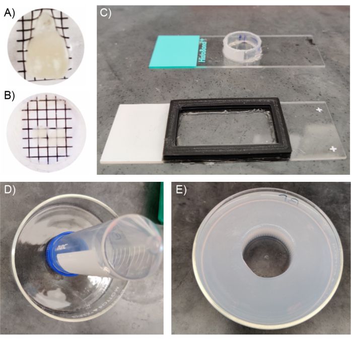
3. Incubate the tissue in the refractive index matching solution (see Table 1) for at least 4 h at room temperature. Figure 1B shows a piece of cleared tissue after incubation in a refractive index matching solution.
4. During the incubation of tissue in refractive index matching solution, construct a suitable housing chamber to image the sample if necessary.
5. Constructing an imaging chamber for small tissue samples/slices
   1. Using a glass slide as a base for mounting, lay down either rubber or plastic spacers and secure with super glue. If premade spacers are not available, use plastic rings made from conical tube cross sections.
   2. Ensure to secure these pieces to the glass slide without any holes (Figure 1C).
   3. Place the cleared tissue into the mounting chamber prefilled with refractive index matching solution.
   4. Securely mount the tissue by placing a glass coverslip on top and sealing it with nail polish.
   5. Image this tissue by adding a drop of refractive index matching mounting solution directly on top of the glass.
6. Large tissue imaging chamber
   1. Construct this chamber if the tissue is larger than 5 mm thick (suitable for whole brains or hemispheres).
   2. Using a 10 cm glass dish with a high wall, place a 50 mL conical tube in the center, making sure that the diameter of conical is large enough to accept the barrel of the objective lens used.
   3. Make 3% agarose in water and pour it in the space between the glass dish and conical tube, allow to cool for 1 h (Figure 1D). This will form a ring of solid agarose (Figure 1E).
   4. Securely adhere the tissue to the bottom of the chamber using super glue and fill the chamber with refractive index matching solution. Apply glue to adhere the tissue on a region that will not be imaged to allow reclamation of the tissue from the dish without damaging the regions of interest.
      NOTE: This preparation is time sensitive, as the refractive index media may start to polymerize unless preserved from air and stored at 4 °C.

2. Imaging cleared tissue samples

1. Acquire the image using a confocal microscope fit with a 25x/0.95 NA objective with a 4 mm working distance.
2. Turn on all the relevant imaging equipment. Place the sample on the stage and place a drop of refractive index matching solution onto the top of the mounting chamber.
3. Carefully approach the immersion media with the objective and form a continuous column of media.
4. Using epifluorescence, find an appropriate imaging field.
5. Begin the image acquisition procedure by testing the appropriate settings.
   1. Start by setting the resolution and scan speed settings using Figure 2A as a guide. If imaging using a confocal microscope, fully close the pinhole to obtain the smallest optical section and thus best z-resolution.
   2. Gradually increase the laser power/sensor gain until a suitable image is obtained with a high signal-to-noise ratio.
   3. If utilizing standard EGFP/tdTomato two-color imaging, set the light collection settings using Figure 2B as a guide.
   4. Set the z-stack parameters based on the observed start and end points of the tissue. Set the step size based on the desired z-resolution using Figure 2C as a guide.
      NOTE: Smaller step sizes will yield a greater z-resolution but will also introduce more laser dwell time, potentially leading to sample bleaching.
   5. When satisfied with image acquisition settings, acquire the image.
   6. Ensure that the image has a high signal-to-noise ratio and shows distinct boundaries of structures (Figure 2D).

3. Image processing and 3D quantification using microscopy analysis software

NOTE: Microscopic image analysis software packages are powerful tools for three-dimensional image visualization and processing. Many of these programs are perfectly suited for the handling of large datasets that are generated from imaging cleared tissue samples. The following steps and associated figures correspond to the Imaris software workflow.

1. Open the image stack and import it into the selected analysis software.
2. View the image in three-dimensional space and make any desired changes to the lookup tables using the display adjuster to better visualize the image.
   NOTE: Figure 3A demonstrates the possible extreme imaging depth accessible through 2-photon microscopy paired with CLARITY tissue clearing. Figure 3B shows distinct dendrite processes as well as clearly visible spine morphologies from the z-stack presented in Figure 3A.
3. To filter out any consistent background, click on the Image Processing button and select the background subtraction filter.
   NOTE: Figure 3C shows the image with a consistent hazy background signal before processing. Figure 3D shows the image after the background subtraction filter has been applied.
4. Observe the 3D image and become familiar with it by looking at it from multiple angles and zoom levels.
5. Start the dendrite tracing by first selecting the Filament tracer tool.
6. Click on Edit the Filament Manually, Skip Automatic Creation.
7. Set the mode to auto path and check Auto-center and Auto-diameter corrections.
8. Shift + right click on the cell body to set a starting point.
9. Trace the neuron along the entire length of the dendrite; left click on the end of the dendrite to set the termination point to allow the software to automatically calculate the path in between the start and end points.
10. Repeat this step for all the dendrites, and fully trace out the cell structure.
11. Visualize the traced cell and confirm its accuracy. Make manual adjustments as needed.
12. Select the Creation tab.
13. Select the Recompute Dendrite Diameter option.
14. Follow the wizard to completion for a more accurately traced dendrite.
15. Select the Draw tab.
16. Click on the Spine radio button to start drawing spines.
17. Set the approximate spine diameter as needed, and use the measurement tool to get an accurate representation of spine diameters.
18. Click on the center of the spine heads to add a new spine.
19. Repeat this for all spines on the dendrite.
    NOTE: It is important to observe the dendrite from all possible angles when manually adding spines.
20. Check the newly added spines for accuracy and make changes as needed.
21. Select the Creation tab.
22. Select the Recompute Spine Diameter option to allow the software to determine the proper head and neck diameters, which are crucial for downstream data analysis.
23. Follow the spine diameter creation wizard to completion.
24. Observe the result of the computation and make any manual adjustments as needed. Figure 3E shows a fully traced neuron complete with spines.
25. To create a classified list of spines, select the Tools tab.
    NOTE: The MATLAB extension must be installed for this to work.
    1. To install the MATLAB extension, open the preferences window.
    2. Select the Custom Tools option.
    3. Add the appropriate MATLAB runtime MCR.
26. Click on Classify Spines.
27. Edit the desired parameters for spine classification.
28. Click on Classify Spines on the MATLAB extension. Figure 3F shows the dendrite overlaid with color-coded classified spines.
29. Select the Statistics tab.
30. Configure the desired statistics to quantify the data by clicking on the Configure button in the bottom-left corner of this tab.
31. Once the method of statistics representation has been chosen, export the data using the Export Statistics on Tab Display to File button located on the bottom right of this window.
32. Graph the statistics using a preferred graphing method.

Results

Materials

List of materials used in this article

Name	Company	Catalog Number	Comments
15 mL Conical Tube	Thermo Scientific	339650
25 G x 1" Needle	BD	305127
30% Acrylamide (No-Bis)	National Diagnostics	EC-810
50 mL Conical Tube	Thermo Scientific	339653
Electrophoretic Tissue Clearing Solution	Logos	C13001
Histodenz	Sigma	D2158-100G
Hydrogel Solution Kit	Logos	C1310X
Imaris	Oxford Instruments	N/A
Paraformaldehyde 16%	EMS	15710
PBS, 1x, 500 mL, 6 bottles/case	fisher	MT21040CV
VA-044	Wako	925-41020
X-CLARITY Polymerization System	Logos	C20001
X-CLARITY Tissue Clearing System II	Logos	C30001