Method Article

Using Spectral Reflectometry to Determine Myelinated Axon Diameters in a Fixed Mouse Brain Slice

656 views

May 29th, 2025

In This Article

Abstract

Source: Kwon, J., et al., Spectral Reflectometric Microscopy on Myelinated Axons In Situ. J. Vis. Exp. (2018)

This video demonstrates the use of spectral reflectometry with a hyperspectral confocal microscope to analyze interference patterns and determine myelinated axon diameters in fixed brain tissue slices.

Protocol

All procedures involving animal samples have been reviewed and approved by the appropriate animal ethical review committee.

1. Calibration

  1. Switch on the microscope at least 1 h before the imaging to allow thermal stabilization of the laser source (see Table of Materials). Then, turn on the software for spectral scanning (see Table of Materials) and click the Acquire button on the top of the GUI (graphical user interface) (Figure 1a).
  2. Turn on the software shutter for the white-light laser (WLL) and photomultiplier tube (PMT) (Figure 1a).
  3. Select the xyΛ mode on the drop-down list in Acquisition Mode, then the laser input mode is automatically changed from Constant percent to Constant Power. Uncheck the checkbox of Automatic SP Movement. Then, set the spectral window of the input laser to 470–670 nm and the spectral step size to 4 nm on Λ-Excitation Lambda Scan Settings (Figure 1b).
  4. SET the spectral range of PMT to 450-690nm by double-clicking or moving the adjustment bar for the spectral range (Figure 1c).
    Note: This spectral range should include the complete bandwidth of the input source.
  5. Select a water-immersion objective lens, suitably with a high numerical aperture (NA > 0.7) and give any value to PMT and laser power to activate AOBS (Acousto-optic beam splitter) configuration and Live Scan button. Switch the optical path by checking the reflection in the AOBS Configuration (Figure 1d).
  6. Mount a reference mirror (see Table of Materials) on the microscope stage. The mirror surface should be facing against the objective lens. If it is not easy to mount the mirror on the microscope stage, bond a mirror onto a flat plate (e.g., slide glass).
  7. Control the microscope stage to align the focal plane to the mirror surface.
  8. Adjust the PMT gain and the laser power, considering the dynamic range of the detector, and then change the laser input mode from Constant Percent to Constant Power.
    Note: As is typical, a PMT gain of 500 (V) and a relative laser power of 0.1% are used at 570 nm.
  9. Confirm in a pseudo-color mode to check that there is no saturation throughout the wavelength range. If saturation is observed, lower the laser power (Figure 1a).
  10. Run the Lambda Scan acquisition.
  11. Remove the mirror from the stage and repeat the same acquisition without a sample in order to obtain the dark reference (i.e., dark offset).
  12. Save the data in a Multistacked TIF format.

2. SpeRe (Spectral reflectometry) Image Acquisition

  1. Place the mounted tissue on the microscope stage. To roughly align the tissue to the focal plane of the objective lens, use the wide-field fluorescence mode through an eyepiece.
  2. With the Live Scan on, control the microscope stage to align the focal plane to the region of interest in the tissue. To avoid the background noise from the coverslip, select the target region of at least 15 μm depth from the glass-tissue interface.
  3. Acquire the spectral image stack for the target region using the same procedure as described in steps 1.1–1.10.
  4. Save the data for the tissue and the dark offset in a Multistacked TIF format.
    Note: The experimenter may pause at this stage.

3. Image Processing and Analysis

  1. Open the spectral data (multi-stacked TIF) for the reference mirror and the brain tissue in ImageJ.
  2. Select the ROIs (regions of interest) for the opened image stacks—the central area for the reference mirror and the segment of an axon fiber for the brain tissue.
  3. Acquire the raw spectra for the selected ROIs by running ImageStacksPlot Z-axis profile on the ImageJ menu.
  4. Open the dark offset data, one taken for the reference mirror and the other taken for the brain tissue.
  5. Acquire the spectra for the dark offsets by running ImageStacksPlot Z-axis profile on the ImageJ menu.
  6. Save all the acquired spectra by using the Copy and Paste options.
    Note: For SpeRe imaging, the use of the central imaging field to minimize off-axis optical aberrations is recommended. The axon fibers may be structurally heterogeneous along their length. Hence, selecting the ROI on a small axon segment, typically < 5 µm, to minimize partial-volume artifact is recommended.

Access restricted. Please log in or start a trial to view this content.

Results
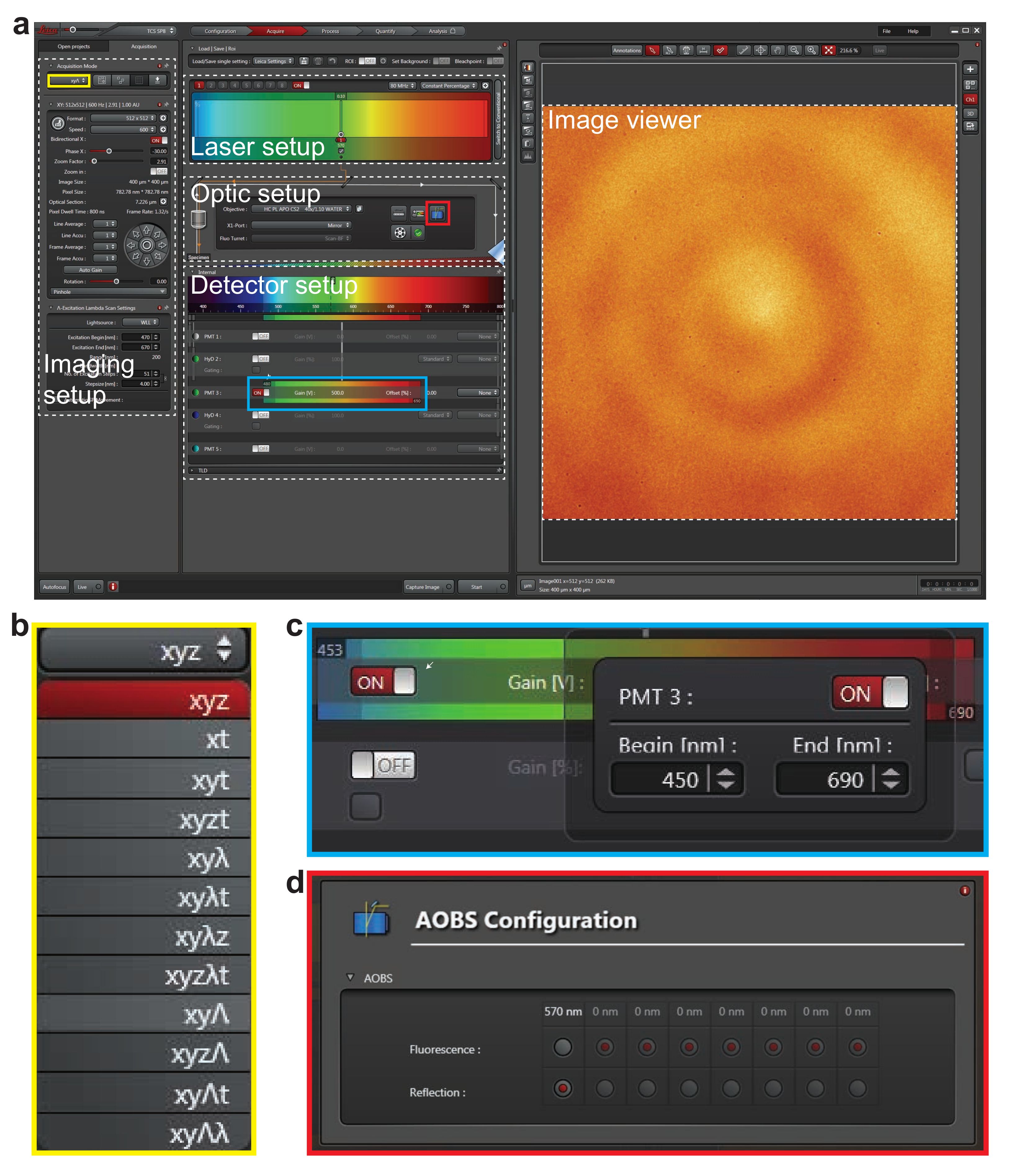
Laser imaging setup interface; optic and detector configuration for microscopy analysis.

Access restricted. Please log in or start a trial to view this content.

Materials

List of materials used in this article
NameCompanyCatalog NumberComments
Apochromat objective 40×, NA 1.1Leica Microsystems15506357Water-immersion type.
Fluoromyelin GreenThermo FisherF34651
Leica SP8 TCS microscopeLeica MicrosystemsSP8
Imaging softwareLeica MicrosystemsLAS-X
MatlabMathWorks
MirrorThorlabsPF10-03-P01Coated with protected silver.
Cover slipThermo Fisher3306Thickness: #1 (0.13 to 0.17 mm).
Slide glassMuto Pure Chemicals5116-20FThickness: ~1 mm.
Super glueHenkelLoctite 406Use a dispensing equipment to avoid skin or eye contact.
White-light laserNKT photonicsEXB-6EXB-6 was discontinued and replaced by EXU-6.

Reprints and Permissions

Request permission to reuse the text or figures of this JoVE article

Request Permission

Tags

Myelinated AxonsAxon Diameter MeasurementFixed Brain SliceHyperspectral MicroscopyConfocal MicroscopeMyelin Sheath AnalysisInterference PatternsReflectance SpectrumImageJ Analysis

Related Articles