Morphological and Physiological Monitoring of Tumor Spheroids Using Optical Coherence Tomography

Abstract

Source: Huang, Y. et. al., Longitudinal Morphological and Physiological Monitoring of Three-dimensional Tumor Spheroids Using Optical Coherence Tomography. J. Vis. Exp. (2019)

This video demonstrates the use of optical coherence tomography (OCT) to monitor tumor spheroids in a multi-well plate by capturing high-resolution cross-sectional images. By analyzing light reflections from cellular structures, OCT constructs 3D models to assess morphological features like size and shape while also distinguishing viable from non-viable cells based on light scattering changes over time.

Protocol

1. Preparation of Cells

1. Obtain cell lines from a qualified supplier.
   NOTE: Verify that cells from the cell lines of interest can form spheroids in the culture media or with the help of a substrate (basement membrane matrix like Matrigel). Look into the literature or perform one round of a pre-experiment for a check.
2. Thaw the frozen cells following the specific procedure provided by the cell-line supplier. A general procedure can be found elsewhere.
3. Culture the cells for 1-2 passages in 25 cm² culture flasks. The cells are then ready to use for 3D cell culture.
4. Monitor the cells' health status daily and maintain them in an incubator under standard conditions (37 °C, 5% CO₂, 95% humidity). Refresh the media as needed.
   NOTE: The culture medium consists of Dulbecco's Modified Eagle medium (DMEM) (4.5 g/L glucose), 1% antibiotic-antimycotic, and 10% fetal bovine serum (FBS). Subculture cells before they reach confluence in the culture flask. Follow the cell culture guidelines provided by the supplier. A general procedure can be found elsewhere.
5. Perform 3D cell culture in multi-well plates based on the following general protocol.
   1. Remove the culture media from the culture flask and wash it with sterilized phosphate-buffered saline (PBS, heated to 37 °C).
   2. Resuspend the cells by adding 1 mL of trypsin ethylenediaminetetraacetic acid (EDTA, 0.5%) into the flask for 3 min. Then, add culture media to dilute the trypsin.
   3. Transfer the cell suspension into a 15 mL centrifuge tube and centrifuge for 5 min at 500 x g and room temperature.
   4. Remove the supernatant and resuspend cells with 4 mL of pre-warmed culture medium. Pipette one drop of the sample onto a hemocytometer for cell counting to determine the cell concentration. Dilute the cells to the appropriate concentration for seeding (e.g., 3,000 cells/mL).
      NOTE: Optimize the spheroid's initial cell concentration for each cell line and each type of multi-well plate (96-well, 384-well, or 1536-well).
   5. Seed cells into an ultra-low attachment (ULA) round-bottomed multi-well plate. Add 200 µL of cell suspension into each well at a concentration of 3,000 cells/mL so that each well has about 600 cells.
   6. At room temperature (RT), centrifuge the whole plate using a plate adapter for 7 min, right after seeding, at a speed of 350 x g or the lowest speed available.
      NOTE: The centrifuge helps gather cells to the center of the well to facilitate forming a single, uniform spheroid. The centrifuge step is performed only once at the beginning to form the tumor spheroids. It will not be repeated when the tumor spheroids start growing.
   7. Maintain the multi-well plate at 37 °C and 5% CO₂ in a culture incubator and refresh the culture media every 3 days.
      NOTE: Growth time may vary for different 3D culture conditions. In our study, 3,000 cells/mL are used for both U-87 MG and HCT 116 cell lines in 96-well plates, so that the spheroid can grow to ~500 μm in 4‒7 days for HCT 116 cells. Based on the general 3D culture protocol, consider adding media supplements and growth factors for different spheroid models.
   8. Perform optical coherence tomography (OCT) imaging of tumor spheroids every 3‒4 days for a longitudinal study of their growth.
      NOTE: The recommended time points for OCT imaging are day 4, day 7, day 11, day 14, day 18, and day 21.

2. High-throughput OCT Imaging Platform

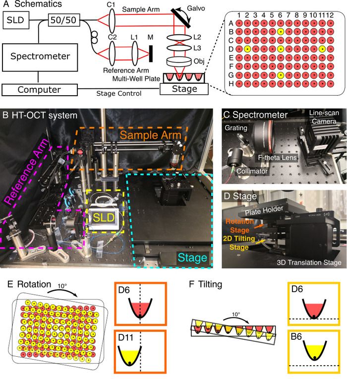
NOTE: See Figure 1 for details of the custom OCT imaging system used in this study.

1. Choose an appropriate broadband light source for the OCT system for tumor spheroid imaging.
   NOTE: Here, a superluminescent diode (SLD, Figure 1A, B) with a central wavelength of ~1,320 nm and a bandwidth of 110 nm was used as a broadband light source.
2. Construct the reference arm and sample arm of the OCT system following the schematics (See Figure 1A, B for details). The Table of Materials lists the optical components needed to construct the OCT system. Ensure that the optical path lengths of the reference arm and sample arm are closely matched.
3. Construct the spectrometer, including a collimator, a grating, an F-theta lens, and a line-scan camera (See Figure 1C for setup) for details of the spectrometer design of OCT. Alternatively, select a commercial spectrometer that matches the center wavelength of the light source. Make sure that the spectrometer is aligned correctly to cover the entire laser bandwidth, to achieve high photon collection efficiency, and to provide slow wash-out of the interference pattern.
4. Characterize the performance of the OCT system, including the following metrics such as sample arm power, total imaging depth, depth-dependent sensitivity, axial resolution, depth of focus, and lateral resolution. Place a weak reflector (e.g., a mirror with a neutral density filter) as a sample to measure the depth-dependent sensitivity, axial resolution, and depth of focus. Place a United States Air Force (USAF) resolution test chart target as the sample to check the lateral resolution.
5. Select a motorized translation stage to provide horizontal movement of the multi-well plate to image tumor spheroids in different wells (See Figure 1B). Use a stage with a travel range larger than 108 mm x 72 mm to ensure a full scanning of all the wells of the multi-well plate. Use a two-dimensional (2D) or three-dimensional (3D) motorized translation stage with software control to enable the precise location of each well and automation of the OCT system for high-throughput imaging.
6. Use a plate adapter or design a plate holder (by 3D printing) to hold the multi-well plate in a fixed position.
7. Before conducting any OCT imaging, correct the tilting and rotation of the multi-well plate using a 2D tilting stage and a rotation stage mounted on the translational stage (See Figure 1D) to minimize variation of the focus plane from different wells. Use D2, D11, B6, D6, and G6 as the guiding wells when monitoring their relative positions in the OCT images (Figure 1A).
8. Adjust the rotation of the plate to ensure the edges are parallel with the direction of stage movement so that the wells remain at the same horizontal positions in the OCT images (Figure 1E). Adjust the tilting of the plate to be parallel to the optical table so that the wells remain at the same vertical locations for OCT imaging (Figure 1F).
   NOTE: Adjustment of the tilting angle and focus helps optimize the OCT image quality for all the wells. However, variations of the height of culture media in different wells may cause changes in optical path,s which may lead to defocusing of the spheroid image. Auto-focus may be implemented to control the focal plane of OCT imaging to achieve optimized image quality. The adjustment step does not resolve poor OCT image quality of the tumor spheroid due to the following issues: the spheroid decentering due to the initial seeding location; spheroid elevation when embedded in biofabricated extracellular matrices; poor plate quality with large variations of the height of well bottoms. Additional software control with auto-focus or self-alignment functions can be implemented to optimize the performance of the OCT imaging system.
9. To collect data from each well sequentially, a custom computer program controls the OCT image acquisition and the stage movement.

3. OCT Scanning and Processing of Tumor Spheroids

1. On the day of the OCT imaging of tumor spheroids, remove the multi-well plate from the incubator. Transfer it under the OCT imaging system and place it on top of the plate adapter.
   NOTE: OCT imaging of tumor spheroids may be performed with the polystyrene plate lid on or off. However, the water condensations on the lid due to evaporation from the wells may affect light transmission and distort the light path, yielding less optimal OCT images from the spheroids.
2. Adjust the height of the plate by moving along the z-direction of the translation stage. Maintain the focal plane position at ~100–200 μm below the top surface of each spheroid, to minimize the effect of the non-uniform depth-wise focal profile.
3. In the custom software, set a proper OCT scanning range (e.g., 1 mm x 1 mm) to cover the whole tumor spheroid according to its development stages. Click Save Parameters to save the setting.
4. Use the custom software to acquire 3D OCT images of tumor spheroids one by one for all the wells of the plate containing spheroids. Click the Preview button to view the preview image and click the Acquire button to acquire the OCT image.
   NOTE: Ensure that the OCT spheroid data are collected when the stage is not in motion. The spheroid is usually located at the center of the U-bottom well. However, the spheroid may be shifted in the culture media when the stage is accelerating or decelerating due to the inertia of the spheroid in the culture media.
5. Process 3D OCT datasets of tumor spheroids to generate OCT structural images with a custom C++ processing code. See Figure 2A for a flowchart of the post-processing of OCT data.
   NOTE: See Figure 3A for the generated 3D OCT structural images.
   1. Calibrate the pixel size in all three dimensions. Rescale the OCT structural images on corrected scales.
      NOTE: The distance in the axial direction (z-direction) of OCT images measures the optical path difference between the reference arm and sample arm. Thus, the refractive index of the sample (n) needs to be taken into consideration when calibrating the pixel size in the axial direction for rescaling. In our study, we use n = 1.37 as the refractive index of the tumor spheroid.
6. Generate a collage of spheroid images using 2D OCT Images in three cross-sectional XY, XZ, and YZ planes across the centroid of the spheroid. See Figure 4C–E for the representative output of collages of spheroid images. Perform image registration for all the spheroids, using the MATLAB function dftregistration, to ensure that the centroids of all the spheroids are located approximately at the same location.
7. Obtain a 3D rendering of the spheroid using commercial or custom software.
   NOTE: The following steps show how to obtain the 3D rendering of tumor spheroids using commercial software.
   1. Load the 3D OCT data into the software.
   2. Click the Surpass panel. Then, click Add New Volume. Choose the Blend mode to use for 3D rendering.
   3. Adjust the viewing angle by dragging the image using the mouse pointer.

4. Morphological Quantification of 3D Tumor Spheroids

NOTE: A custom-written code in MATLAB processes this quantification. Click the Run button to initiate the process. See Figure 2B for the flowchart of the steps of morphological quantification of spheroids.

1. Quantify spheroid diameter, height, and diameter-based volume.
   1. Select 2D OCT Images in three cross-sectional XY, XZ, and YZ planes that cross the centroid of the spheroid.
   2. Measure the diameter and height of the spheroid in XY and XZ planes, respectively.
   3. Calculate diameter-based spheroid volume using:

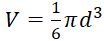
, with a presumption of the spherical shape of the tumor.

2. Quantify voxel-based spheroid volume.
   1. Apply a 3D averaging filter on the OCT structural data of the spheroid to remove speckles.
   2. Segment tumor spheroids using the Canny edge detection filter, frame by frame, with a proper threshold separating the tumor spheroid region from the well bottom.
   3. Group connective voxels for 3D data (see built-in function: bwconncomp).
   4. Calculate the mean distance between each connective voxel in the group and the spheroid centroid (manually chosen), for each group. Identify the spheroid region as the group with the minimum mean distance.
   5. Count the number of voxels within the spheroid region and then multiply by the actual volume of an individual voxel (volume/voxel), yielding the total volume of the spheroid.

5. Dead-Cell Region Detection of 3D Tumor Spheroids

NOTE: In a homogeneous medium, OCT back-scattered intensity detected as a function of depth (I(z)) can be described by the Beer-Lambert Law:

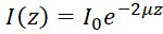
Where z represents the depth, μ is the optical attenuation coefficient, and I0 is the incident intensity to the sample. Hence the derived optical attenuation coefficient can be expressed as:

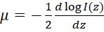
Since OCT images are often plotted on a logarithmic scale, the slope of the OCT intensity profile can be retrieved to derive the optical attenuation coefficient. See Figure 2C for a flowchart of the generation of the optical attenuation maps.

1. Perform segmentation to remove unwanted regions outside the spheroid. Perform a 3D average filter to suppress the speckle noise that is inherent in OCT images.
2. Obtain pixel-wise optical attenuation coefficients by linear fitting the log-scale OCT intensity profile over a certain depth range (moving window), extracting its slope, and multiplying the slope by -1/2.
   NOTE: The attenuation coefficient at each voxel within the segmented spheroid region is calculated based on the slope of the OCT intensity profile in a 10-voxel depth window (~40 μm in depth), with the voxel located in the middle of the window.
3. Apply the methods above (steps 5.1 and 5.2) to each axial scan in a frame and each frame in a 3D dataset containing the segmented spheroid region until optical attenuation coefficients for all voxels of the segmented spheroid region are calculated.
4. Perform the binary thresholding to highlight the high-attenuation region.
   Highlight the binarized optical attenuation map on the original image to label the dead-cell region (blending). Generate the 3D-rendered image of the blended attenuation map to visualize the 3D distribution of the dead-cell region.

Results

Materials

List of materials used in this article

Name	Company	Catalog Number	Comments
Custom Spectral Domain OCT imaging system			Developed in our lab
Superluminescent diode (SLD)	Thorlabs	SLD1325	Light source
2×2 single mode fused fiber coupler, 50:50 splitting ratio	AC Photonics	WP13500202B201
Reference Arm
Lens Tube	Thorlabs
Adapter	Thorlabs
Collimating Lens	Thorlabs	AC080-020-C
Focusing Lens	Thorlabs
Kinematic Mirror Mount	Thorlabs
Mirror	Thorlabs
1D Translational Stage	Thorlabs
Continuous neutral density filter	Thorlabs
Pedestrial post	Thorlabs
Clamping fork	Thorlabs
Sample arm
Lens tube	Thorlabs
Adapter	Thorlabs
Collimating lens	Thorlabs	AC080-020-C
Galvanometer	Thorlabs
Relay lens	Thorlabs	AC254-100-C	Two Relay lens to make a telescope setup
Triangle mirror mount	Thorlabs
Mirror	Thorlabs
Objective	Mitutoyo
Pedestrial post	Thorlabs
Clamping fork	Thorlabs
Polarization controller	Thorlabs
30mm cage mount	Thorlabs
Cage rod	Thorlabs
Stage
3D motorized translation stage	Beijing Mao Feng Optoelectronics Technology Co., Ltd.	JTH360XY
2D Tilting stage
Rotation stage
Plate holder			3D printed
Spectrometer
Lens tube	Thorlabs
Adapter	Thorlabs
Collimating lens	Thorlabs	AC080-020-C
Grating	Wasatch		G = 1145 lpmm
F-theta lens	Thorlabs	FTH-1064-100
InGaAs line-scan camera	Sensor Unlimited	SU1024-LDH2
Cell Culture Component
HCT 116 Cell line	ATCC	CCL-247
Cell culture flask	SPL Life Sciences	70025
Pipette	Fisherbrand	14388100
Pipette tips	Sorenson Bioscience	10340
Gibco GlutaMax DMEM	Thermo Fisher Scientific	10569044
Fetal bovine serum, certified, US origin	Thermo Fisher Scientific	16000044
Antibiotic-Antimycotic (100X)	Thermo Fisher Scientific	15240062
Corning 96-well clear round bottom ultra-low attachment microplate	Corning	7007
Gibco PBS, pH 7.4	Thermo Fisher Scientific	10010023
Gibco Trypsin-EDTA (0.5%)	Thermo Fisher Scientific	15400054
Forma Series II 3110 Water-Jacketed CO2 incubator	Thermo Fisher Scientific	3120
Gloves	VWR	89428-750
Parafilm	Sigma-Aldrich	P7793
Transfer pipets	Globe Scientific	138080
Centrifuge	Eppendorf	5702 R	To centrifuge the 15 mL tube
Centrifuge	NUAIRE	AWEL CF 48-R	To centrifuge the 96-well plate
Microscope	Olympus
List of Commerical OCTs
SD-OCT system	Thorlabs	Telesto Series
SD-OCT system	Wasatch Photonics	WP OCT 1300 nm
Software for Data Analyses
Basic Image Analysis	NIH	ImageJ	Fiji also works.
3D Rendering	Thermo Fisher Scientific	Amira	Commercial software. Option 1
3D Rendering	Bitplane	Imaris	Commercial software. Option 2. Used in the protocol
OCT acquisition software			custom developed in C++.
Stage control	Beijing Mao Feng Optoelectronics Technology Co., Ltd.	MRC_3	Incorporated into the custom OCT acquisition code
OCT processing software			Custom developed in C++. Utilize GPU. Incorporated into the custom OCT acquisition code.
Morphological and Physiological Analysis			Custom developed in MATLAB