Fluorescence Lifetime Imaging of PolyQ Protein Aggregation in Caenorhabditis elegans Neurons

Abstract

Source: Pigazzini, M. L., et. al. Characterization of Amyloid Structures in Aging C. Elegans Using Fluorescence Lifetime Imaging. J. Vis. Exp. (2020).

This video demonstrates the use of fluorescence lifetime imaging microscopy (FLIM) to assess polyQ protein aggregation in C. elegans neurons, comparing control and chaperone protein-deficient worms. Increased aggregation in chaperone-deficient worms promotes energy transfer between clustered fluorophores, reducing fluorescence lifetime. FLIM-generated color-coded maps depict these differences, highlighting aggregation levels between experimental groups.

Protocol

1. Acquisition of FLIM data

NOTE: In this protocol, the lifetime of the fluorophore is acquired via the time-domain TCSPC method. FLIM requires a pulse of light to be generated by the laser at a set and constant repetition rate. The repetition rate varies according to the laser type and needs to be known by the user. Lifetime measurements are achieved by detectors and electronic equipment installed alongside a conventional microscope. In this protocol, measurements are performed on three different laser scanning confocal microscopes with detectors and software provided by two different companies (Table of Materials) for acquisition of mRFP, CFP, and YFP lifetimes, respectively. Check that the correct filters of emission/excitation are in place and minimize any background or monitor backlight before starting. Before starting any experiment, establish the photostability of the chosen fluorophore. If the fluorophore bleaches within a short time within the nematode tissues, it is not suitable for FLIM measurements in C. elegans.

1. Open the FLIM acquisition software. The FLIM software also allows control of the confocal microscope. Locate the tab/button to allow for the detector's outputs to be enabled and press Enable Outputs.
2. Acquire the instrument response function (IRF), which describes the timing precision of the instrumental setup.
   NOTE: This step should be performed preferably before mounting the nematodes.
   1. If available, remove the excitation/emission filters.
   2. Place an empty coverslip above the objective and find its surface. Record the scatter signal obtained from the coverslip for a minimum of 30 s.
      NOTE: For lifetimes of several nanoseconds, the acquisition software can automatically estimate the IRF shift. Acquiring an IRF is always recommended.
3. Place the slide with the mounted C. elegans on the stage. Using a 10x magnification lens in transmission mode and localize the position of the nematodes on the slide.
4. Remove the slide, switch the objective to a 63x magnification lens, and apply the required immersion medium (e.g., oil). Replace the slide on the stage and localize the nematodes.
5. Locate the Pinhole Manager on the acquisition software and open it to the Maximum. Start scanning the sample, select a region of interest (e.g., head, upper body), and focus on its maximum projection plane.
6. Monitor the laser pulse rate and the three other values present on the interface of the software: The Constant Fraction Discriminator (CFD), the Time-to-Amplitude (TAC), and the Analogue-to-Digital Converter (ADC).
   NOTE: The laser should have a maximum gate of 1 x 10⁸ single photon counts. This number represents the maximum number of photons supplied by the laser. The CFD provides information on the receipt of the single photon pulse in reference to the laser pulse by the detector. This value should be roughly 1 x 10⁵. The TAC discriminates between the time one photon was detected and the next laser pulse. Finally, the ADC converts the TAC voltage into a storable memory signal. The CFD, TAC, and ADC should all have similar values to ensure that photons emitted by the fluorophore are not lost. Correct evaluation of these parameters ensures that enough photons are being collected to create an accurate lifetime map.
7. On the interface of the FLIM software, preview the number of photons detected: the ADC value should be between 1 x 10⁴ and 1 x 10⁵. If necessary, shift the focus on a different plane or increase the laser power to collect more photons.
   NOTE: In general, the number of recorded photons per second should not exceed 1% of the laser's repetition rate.
8. In the menu bar, select the tab to set the acquisition parameters. Select scan sync in to allow for single photon detection.
9. Set the acquisition to a fixed amount of time or a fixed number of photons. For example, acquire a lifetime decay curve for 2 min or until a single pixel reaches a photon count of 2,000 single events. Press Start to begin acquisition.
   NOTE: Different fluorophores will require different excitation and emission lasers and filters. According to the brightness of the sample, the laser power can also be adjusted, which will not interfere with the lifetime. These protocols use the following excitation/emission settings: YFP ex500/em520-50 nm, mRFP ex561/em580-620 nm. A pulsed two photon laser was employed for CFP measurements using ex800/em440 nm. The amount of time and photon count required for acquisition of a FLIM map will need to be empirically established for each setup and each experimental purpose.

2. Analysis of FLIM data using FLIMfit software

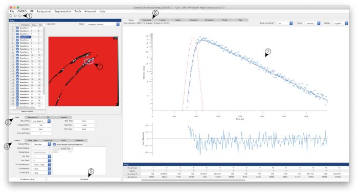
NOTE: Perform data analysis using the FLIMfit software tool developed at Imperial College London (see Figure 1).

1. Open the software and import FLIM data files via File | Load FLIM Data. Load all samples from one condition, even if obtained in different sessions and from different biological repeats.
2. If necessary, segment a single nematode from any FLIM picture via Segmentation | Segmentation Manager. Drag the cropping tool around the area of interest until it is highlighted. Once completed, press OK.
   NOTE: Segmentation must be done for all images.
3. Select a small region where the intensity-based image of a C. elegans appears (Figure 1, Arrows 1). The decay curve of that region will appear in the large decay window on the right side of the interface (Figure 1, Arrow 2).
   NOTE: The decay can be displayed linearly or logarithmically.
4. Set the correct parameters to extrapolate the lifetime via the software's algorithm as described in steps 2.5-2.8.
5. On the Data tab (Figure 1, Arrow 3):
   1. Set an arbitrary Integrated Minimum value to exclude any pixels that are too dim to produce a good fit. Depending on the C. elegans sample this value varies from 40-300. Input different values until a satisfactory preview is achieved.
   2. Select a Time Min and a Time Max number to limit the FLIM signal to these values. All events that appear before and after this threshold will be excluded.
      NOTE: For example, for the analysis of mRFP, the events prior to 800 ps and after 4,000 ps were excluded. These values depend on the lifetime of the fluorophore and need to be determined by the end user.
   3. Do not change the preset Counts/Photon of 1.
   4. Input the Repetition Rate, in MHz, of the laser utilized during acquisition.
      NOTE: For the current protocol, different lasers were utilized with various repetition rates. The two photon laser used for acquisition of CFP lifetimes possesses a repetition rate of 80 MHz, for YFP the laser repeats at 40 MHz, and for mRFP the value is 78.01 MHz. These values were inputted into FLIMfit according to the sample analyzed.
   5. Input a Gate Max value to exclude all saturated pixels.
      NOTE: For lifetime measurements in C. elegans, this value is set to any large number (e.g., 1 x 10⁸).
6. On the Lifetime tab, select a global fitting to be used (e.g., a pixel-wise fitting). See Figure 1, Arrow 4.
   NOTE: A Pixel-wise fitting will produce a decay fitted to each individual pixel. An Image-wise fitting will produce a global fitting of each individual image and display a single lifetime value per image. A Global-wise fitting will produce a single fitting across the whole dataset. A single lifetime value is provided for all images.
7. Do not change any other parameter except for the No. Exp selection if it is known that the chosen fluorescence decay is multiexponential and exhibits more than a single lifetime.
   NOTE: In the present protocol, this function was utilized to calculate the lifetimes of the biexponential CFP fluorophore.
8. Upload the IRF via the IRF menu: IRF | Load IRF. To estimate the IRF shift, select IRF | Estimate IRF Shift. A set of values will automatically appear on the IRF tab. Once this is established, do not change any other parameters of this tab.
9. Once all parameters are set, press Fit Dataset (Figure 1, Arrow 5). The algorithm will produce a fit for the decay curve and establish a lifetime value for each image.
   NOTE: The resulting fit, highlighted in a blue line, should overlap with all the events. A good fit is obtained when all events are aligned along the fit.
10. Click the Parameters tab (Figure 1, Arrow 6), located within the top right menus of the software's interface, and select Statistic: w_mean (weighted mean) and check that the chi2 value is as close as possible to 1.
    NOTE: A chi2 close to one ensures the accuracy of the fit. The lifetime value of the selected image is thus revealed as tau_1.
11. Export any information of interest: File | Export Intensity Images/Fit Result Table/Images/Histograms. Save the data settings used to calculate the lifetime: File | Save Data Settings.
    NOTE: The parameters employed will be saved for future analysis of the selected samples.

3. Graphical representations of FLIM data

NOTE: The lifetimes collected from different samples can be visually represented in various ways. Select to denote the lifetime values either in nanoseconds or picoseconds.

1. Show the quality of the fit and the accuracy of the curve by exporting the decay curve directly from FLIMfit.
2. Represent the distribution of the photons by plotting the frequency of the photon count versus the lifetime value in a histogram.
3. Finally, for statistical comparison, if comparing two or more samples, place lifetime values plus standard deviation of the mean in a scatter plot bar graph. Perform any desired statistical analysis.

Results

Materials

List of materials used in this article

Name	Company	Catalog Number	Comments
Ampicillin	Carl Roth GmbH + Co. KG	K029.3	Antibiotic
B&H DCS-120 SPC-150	Becker & Hickl GmbH		FLIM Aquisition software
B&H SPC830-SPC Image	Becker & Hickl GmbH		FLIM Aquisition software
C. elegans nQ40-CFP			Kind gift from Morimoto Lab
Deckgläser-18x18mm	Carl Roth GmbH + Co. KG	657.2	Cover slips
Leica M165 FC	Leica Camera AG		Mounting Stereomicroscope
Leica TCS SP5	Leica Camera AG		Confocal Microscope
Levamisole Hydrochloride	AppliChem GmbH	A4341	Anesthetic
PicoQuant PicoHarp300	PicoQuant GmbH		FLIM Aquisition software
Sodium Azide	Carl Roth GmbH + Co. KG	K305.1	Anesthetic
Standard-Objektträger	Carl Roth GmbH + Co. KG	656.1	Glass slides
Universal Agarose	Bio & Sell GmbH	BS20.46.500
Zeiss AxioObserver.Z1	Carl Zeiss AG		Confocal Microscope
Zeiss LSM510-Meta NLO	Carl Zeiss AG		Confocal Microscope