Developing a Cerebral Blood Flow Atlas for Blood Flow Mapping

Abstract

Source: Tan, Z., et al., Construction and Application of Cerebral Functional Region-Based Cerebral Blood Flow Atlas Using Magnetic Resonance Imaging-Arterial Spin Labeling. J. Vis. Exp. (2024).

This video demonstrates the method to construct a cerebral blood flow atlas by integrating magnetic resonance imaging or MRI-arterial spin labeling data with segmented brain regions, visualizing blood flow patterns, and quantifying flow levels across functional areas.

Protocol

1. Data collection and preparation

NOTE: The variance in parameters remains unaffected by the research approach. Both digital imaging and communications in medicine (DICOM) and neuroimaging informatics technology initiative (NIFTI) formats are used for storing digital medical imaging data, with DICOM being the usual output from clinical imaging devices. However, the NIFTI format is often preferred for computational convenience in research activities. Converting from DICOM to NIFTI is a straightforward and common practice. In this study, authentic DICOM data were acquired and converted into NIFTI format. The data was acquired using a 1.5 Tesla magnetic resonance imaging (MRI) scanner. In the cross-image registration process of this study, the fluid-attenuated inversion recovery (FLAIR) sequence was mainly used and fused with cerebral blood flow (CBF) images. The CBF Atlas tool (Table of Materials) used in this study is commercial software.

1. Copy data to the designated working directory.
   1. Copy all NIFTI data to a customized working directory.
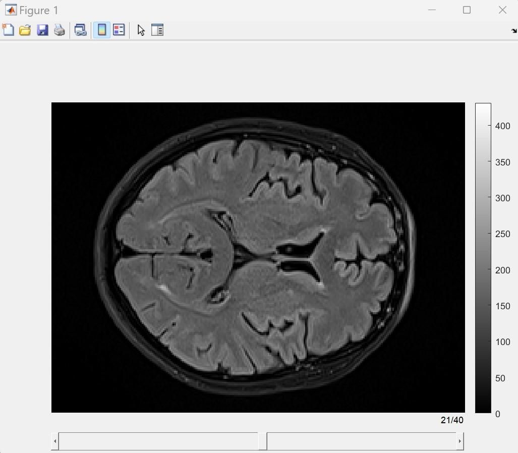
      NOTE: The working directory is the same in the operating system and matrix laboratory (MATLAB). The research follows the right anterior superior (RAS) orientation standard.
   2. Go to the directory housing the data within MATLAB's current working directory, and use the niftiread function to load FLAIR data into the workspace. Use the size function to check the dimensions of the FLAIR sequence. Call the Flair_Slice command to view the FLAIR sequence (as shown in Figure 1). Use the specific commands as follows:
      FLAIR_XLF = niftiread('FLAIR_XFL.nii');
      size(FLAIR_XLF)
      ​Flair_Slice(FLAIR_XLF);
   3. Refer to Figure 1 for an image of the interactive graphic user interface (GUI) for the FLAIR sequence. Use the bottom scroll bar to quickly browse the different sequences.
2. Quickly check images of CBF.
   1. Use the niftiread function to load CBF data into the workspace. Use the size function to check the dimensions of the CBF sequence. Call the CBF_Slice command to view the CBF sequence (as shown in Figure 2). Use the specific commands as follows:
      CBF_XLF = niftiread('CBF_XFL.nii');
      size(CBF_XLF)
      CBF_Slice(CBF_XLF);
   2. Refer to Figure 2 for an interactive GUI screenshot of the CBF sequence. Use the bottom scroll bar to quickly browse the different sequences.
      NOTE: In Figure 2, the CBF value range is usually 0-120 mL/100 g/min. Figure 2 uses a color map to represent different CBF levels in different colors.

2. Segmentation of cerebral functional regions from the FLAIR sequence

NOTE: The FLAIR sequence serves as both structural imaging and provides excellent pathological diagnostic capabilities. Therefore, fusing FLAIR with CBF holds important diagnostic value in clinics. This study segments major cerebral functional regions from the FLAIR sequence.

1. In the workspace, call the FLAIR_Segment function and run the pretrained 3-D U-Net-based image segmentation program to automatically generate triplanar views of cerebral functional regions segmentation, as shown in Figure 3. Each color in Figure 3 represents a distinct functional region.
2. For real-time inspection of different cerebral functional regions, use the crosshair interaction (Figure 3). Click and drag the center of the crosshair for an arbitrary 3D examination of the reconstructed brain anatomy.
   NOTE: The GUI in Figure 3 also enables adjustment of the grayscale intensity range, contrast, and brightness of the triplanar views.
3. Press and drag the left mouse button over any region of the images to modify brightness and contrast levels in real time. Release the mouse button to confirm and finalize the adjustments.

3. Triplanar views of CBF distribution across cerebral functional regions

NOTE: Examining CBF distribution across different cerebral functional regions facilitates precise clinical judgments of patient conditions. Under the functional region framework from Figure 3, incorporating the exact CBF values from the CBF sequence and presenting them in triplanar views allows comprehensive physician inspection.

1. Call the CBF_triplanar function to generate the triplanar GUI view shown in Figure 4, displaying CBF spatial distribution across functional regions. Move the crosshair to allow examination of CBF distribution in regions of interest.
2. Click the Data Tips button on the top right corner of the GUI to display the CBF values at any position.
3. Press and drag the left mouse button over any region of the images to modify brightness and contrast levels in real time. Release the mouse button to confirm and finalize the adjustments.

4. CBF atlas across major cerebral functional regions

NOTE: Normalizing the CBF probability distributions across different functional regions generates the Cerebral Functional Regions CBF Atlas, expressing the CBF levels across cerebral functional regions of the subject.

1. Call the CBF_Atlas function to convert the CBF spatial distribution shown in Figure 4 into a CBF Atlas (as shown in Figure 5).
   NOTE: In Figure 5, the x-axis represents different cerebral functional regions, and the y-axis represents different CBF levels; the different colors denote different probability levels (the redder the color, the more voxels present).
2. To scale partial images, click the Zoom In/Out button at the top right of the GUI shown in Figure 5.
   NOTE: The curve in Figure 5 connects the average CBF across regions.

Results

Materials

List of materials used in this article

Name	Company	Catalog Number	Comments
CBF Atlas	Intelligent Entropy	CBF Atlas V1.0	Beijing Intelligent Entropy Science & Technology Co Ltd. Modeling for Thyroid Disease
MATLAB	MathWorks	2023B	Computing and visualization
MRI Device	Siemens	Amria 1.5 T	MRI scanner