Detection of Architectural Distortion in Prior Mammograms via Analysis of Oriented Patterns

Summary

We demonstrate methods for the detection of architectural distortion in prior mammograms. Oriented structures are analyzed using Gabor filters and phase portraits to detect sites of radiating tissue patterns. Each site is characterized and classified using measures to represent spiculating patterns. The methods should assist in the detection of breast cancer.

Abstract

We demonstrate methods for the detection of architectural distortion in prior mammograms of interval-cancer cases based on analysis of the orientation of breast tissue patterns in mammograms. We hypothesize that architectural distortion modifies the normal orientation of breast tissue patterns in mammographic images before the formation of masses or tumors. In the initial steps of our methods, the oriented structures in a given mammogram are analyzed using Gabor filters and phase portraits to detect node-like sites of radiating or intersecting tissue patterns. Each detected site is then characterized using the node value, fractal dimension, and a measure of angular dispersion specifically designed to represent spiculating patterns associated with architectural distortion.

Our methods were tested with a database of 106 prior mammograms of 56 interval-cancer cases and 52 mammograms of 13 normal cases using the features developed for the characterization of architectural distortion, pattern classification via quadratic discriminant analysis, and validation with the leave-one-patient out procedure. According to the results of free-response receiver operating characteristic analysis, our methods have demonstrated the capability to detect architectural distortion in prior mammograms, taken 15 months (on the average) before clinical diagnosis of breast cancer, with a sensitivity of 80% at about five false positives per patient.

Introduction

Breast cancer is a major disease affecting women and is the second leading cause of cancer related death among women ^1,2. In order to improve the chance of survival and the prognosis of the affected patients through effective treatment at early stages of breast cancer, the disease needs to be detected as early as possible. In retrospective analysis of cases of breast cancer, subtle signs of abnormalities have been observed on previously acquired screening mammograms ^3,4. Architectural distortion is one such localized mammographic sign of possibly early stages of breast cancer that is difficult to detect ^5,6. The associated patterns are vaguely described as distortion of the normal architecture of the breast with no definite mass visible. Architectural distortion could appear at the initial stages of the formation of a breast mass or tumor. We hypothesize that screening mammograms obtained prior to the detection of breast cancer could contain subtle signs of early stages of breast cancer, in particular, architectural distortion.

Figure 1a shows a prior mammographic image of a case of screen-detected cancer. The region of abnormality identified by a radiologist (J.E.L.D.) is outlined with a red rectangle. The prior mammogram was taken 24 months before the detection mammogram shown in Figure 1b. The prior mammogram had been declared to be free of signs of cancer at the original instance of screening. In retrospective analysis and in comparison with the detection mammogram, a suspicious region related to the site of cancer detected was labeled by the radiologist, and is outlined in red on the prior mammogram. The suspicious region contains signs of architectural distortion, including spicules.

Computer-aided diagnosis (CAD) techniques and systems offer the potential for achieving increased sensitivity in the detection of breast cancer ^2,7-9. However, in comparison with the number of publications that exist in the literature on the detection of other signs of breast cancer, such as masses and calcifications, only a small number of studies have been reported on the detection of architectural distortion in the absence of a central mass ^10-17. Commercially available CAD systems have been found to perform poorly in the detection of architectural distortion ¹⁸. Studies on the detection of architectural distortion in prior mammograms of screen-detected or interval-cancer cases ^3,4,19-22 could help in developing strategies for the detection and treatment of breast diseases at their early stages, and lead to improvement in the prognosis for the patient ²³.

Preparation of Images for the Experiment

Experiments were conducted with 158 mammographic images including 106 prior mammograms of 56 individuals diagnosed with breast cancer and 52 images of 13 normal individuals. Ethics approval for the study was obtained from the Conjoint Health Research Ethics Board, Office of Medical Bioethics, University of Calgary, and the Calgary Regional Health Authority. The images were obtained from Screen Test: Alberta Program for the Early Detection of Breast Cancer ^21,24,25.

Mammograms acquired in the last scheduled visit to the screening program prior to the diagnosis of cancer outside the screening program were labeled as prior mammograms of interval-cancer cases. The corresponding diagnostic mammograms were not available. All but two of the 106 prior mammograms had been declared to be free of any sign of breast cancer at the time of their acquisition and analysis in the screening program; the individuals corresponding to the other two mammograms had been referred for biopsy. The time interval between the diagnosis of cancer and prior mammograms ranged from 1.5 months to 24.5 months, with an average of 15 months and standard deviation of 7 months. All of the prior mammograms of interval-cancer cases available in the database have been included in the present study, except six images in which no suspicious parts could be identified.

The screen-film mammograms were digitized at the spatial resolution of 50 μm and gray-scale resolution of 12 bits per pixel using the Lumiscan 85 laser scanner (Lumisys, Sunnyvale, CA). An expert radiologist specialized in mammography (J.E.L.D.) reviewed all of the 106 prior mammograms of interval-cancer cases and marked the suspected regions of architectural distortion with rectangular boxes based on the reports available on subsequent imaging or biopsy, or by detailed inspection of the mammograms. Of the 106 prior mammographic images in the dataset used in the present study, 38 images have visible architectural distortion, and the remaining 68 images contain questionable or no clearly evident architectural distortion. Each prior mammogram contains a single site of architectural distortion as identified by the rectangular box drawn by the radiologist. The average width, height, and area of the 106 suspicious parts of images marked by the radiologist are 56 mm, 39 mm, and 2,274 mm², with standard deviation of 11.8 mm, 11.6 mm, and 1073.9 mm², respectively.

Protocol

1. Overview of Methodology

In our procedure, potential sites of architectural distortion in mammograms are automatically detected via analysis of oriented textural patterns with the application of a bank of Gabor filters ²⁶ and modeling of phase portraits ^11,27. The detected sites are then processed through the steps of extraction of features or measures to characterize architectural distortion, development of a trained classifier, and application of an algorithm for pattern recognition or classification. The procedure is summarized by the following steps ^11,20,21:

1. Segment the breast portion in the given mammographic image using adaptive thresholding and morphological opening.
2. Apply a set of 180 Gabor filters with angles spaced evenly over the range -90° to +90° to obtain the Gabor magnitude image, M (i, j), and the Gabor angle image, θ (i, j), by selecting the response and angle of the filter with the highest response at each pixel, (i, j).
3. Select curvilinear structures (CLSs) of interest, such as spicules and fibroglandular tissue, by distinguishing them from confounding structures, such as edges of the pectoral muscle, parenchymal tissue, breast boundary, and noise, by using the orientation field, the gradient field, the nonmaximal suppression (NMS) technique, and additional conditions ¹¹.
4. Filter the orientation field with a Gaussian filter with the standard deviation of 7 pixels and down-sample by a factor of four to reduce noise and further computational requirements ^11,20.
5. Apply linear phase-portrait modeling, with a sliding analysis window of size 10 x 10 pixels at 800 μm/pixel, with one pixel per step, to the filtered orientation field, with specific conditions to select phase-portrait maps related to particular types of node patterns ^11,20.
6. Cast a vote, if certain conditions are met, at the position given by the fixed point for each position of the analysis window to form the node map.
7. Filter the node map with a Gaussian window of size 35 x 35 pixels, with the empirically determined standard deviation of 6 pixels (4.8 mm), to consolidate votes in close proximity to one another.
8. Analyze the node map by rank-ordering the peaks in the node map.
9. Cut regions of interest (ROIs), of size 128 x 128 pixels except at the edges, from the original image, with the center of each ROI located at the center of the related peak in the node map. At the edges of the image being processed, create ROIs to include as much of the image data as available in the specified window.
10. Derive features or measures to characterize the spiculating patterns related to architectural distortion and separate them from normal tissue patterns that met some of the initial conditions.
11. Develop a trained classifier to discriminate between the features of sites with architectural distortion and those of normal tissue patterns using a training set of ROIs classified by a radiologist.
12. Apply the trained classifier to a set of test cases and verify the results with diagnosis provided by the radiologist and based on biopsy.

Steps 1-9 listed above are applied automatically to a given mammographic image. Selected steps of the procedure listed above are described and illustrated in the following sections.

2. Preprocessing of Mammographic Images

The preprocessing stage consists of the following steps:

1. Filter the given mammographic image using a Gaussian filter, with a standard deviation of 2 pixels and size of 13 x 13 pixels at the resolution of 50 μm/pixel and 12 bits/pixel, and down-sample to 200 μm/pixel and 8 bits/pixel resolution.
2. Reflect the image if it is of the right breast.
3. Segment the breast region in the mammographic image using Otsu's adaptive thresholding method and morphological opening with a disk-shaped structuring element of radius 25 pixels (5 mm at 200 μm/pixel) ^21,28,29.
4. Detect the approximate breast boundary ^10,21.

Figure 2A shows an original prior mammogram. Figure 2B of the same figure shows the result of approximate segmentation of the breast portion, which is used in the subsequent steps of processing and analysis.

3. Extraction of Oriented Patterns Using Gabor Filters

The real Gabor filter function oriented at -90° is specified in our work as ^10,30:

where σ_x and σ_y are the standard deviation values in the x and y directions, and ƒ_o is the frequency of the modulating sinusoid. Filters at other angles are obtained by rotating this function using coordinate transformation as:

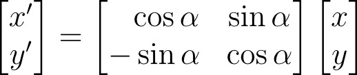
where (x', y') is the set of coordinates rotated by the angle α.

The parameters in Equation 1 for filtering mammograms are derived in our work by taking into account the average size of the breast tissue patterns to be detected, as follows ¹⁰:

1. Let Τ be the full-width at half-maximum of the Gaussian term in Equation 1 along the x axis.
2. Let Τ = 4 pixels, corresponding to a thickness of 0.8 mm at the pixel size of 200 μm.
3. Calculate .
4. Let the period of the cosine term be Τ; then, ƒ_o= 1/Τ.
5. Let the value of σ_y be defined as σ_y = lσ_x, where l determines the elongation of the Gabor filter in the y direction, as compared to the width of the filter in the x direction. For analysis of mammograms at 200 μm/pixel, use l = 8.

A bank of 180 real Gabor filters evenly spaced over the range -90° to +90° is used in our methods for the detection of oriented patterns in mammograms ^{10, 21}. For each given image, a Gabor magnitude image, M(i, j), and a Gabor angle image, θ(i, j), are obtained using the response and angle of the Gabor filter with the highest response at each pixel, (i, j).

The Gabor filter has a nonzero magnitude response at the origin of the frequency plane (zero frequency). Because low-frequency components are not related to the presence of architectural distortion, it is desirable to reduce the effect of the low-frequency components of the mammographic image in the orientation field magnitude. Therefore, the mammographic images are high-pass filtered prior to the extraction of the orientation field. This is achieved by computing the difference between the original image and a low-pass-filtered version of the same image. The low-pass filter used in this step is a Gaussian filter with the standard deviation equal to σ_y defined as above.

Although one could save the filtered image for each angle of interest, in the present work, the maximum response at each pixel over all of the filters (angles) used is saved in a single image, referred to as the Gabor magnitude response; the corresponding angle of the Gabor filter is saved at each pixel in another image, referred to as the Gabor angle response. Together, the two output images provide the orientation field of the given image.

Figure 3A shows a test image of a plant. Figure 3B shows the Fourier spectrum of the image, which depicts concentrations of energy at various angles. All parts of the image with the same orientation, regardless of their position and size, have their frequency components (spectral energy) located in an angular band or sector positioned at 90° with respect to their orientation in the image. The results of filtering the image with Gabor filters with Τ = 8 pixels and l = 8 are shown in Figures 3C and D. It is evident that the Gabor filters have extracted parts of the plant oriented at various angles with high magnitude response and that the angle response agrees with the orientation of the dominant feature present at the corresponding pixel. By using a bank of Gabor filters oriented at several angles over the range -90° to +90°, we have extracted all of the oriented components present in the image and their angles at each pixel. It is evident that the response of the Gabor filters is almost zero in smooth areas with the same intensity level and no structures with preferred orientation, such as parts of the pot and the wall.

Figure 4 shows the Gabor magnitude and angle responses obtained for the mammogram with architectural distortion shown in Figure 2B. It is evident that the Gabor filters have extracted oriented components with high responses as well as the corresponding angles. It is also seen that the response of the Gabor filters is low in smooth areas with almost constant density and no structures with preferred orientation. Upon close inspection, it may also be observed that the response of the Gabor filters depends upon the contrast of an oriented structure in relation to its background and not only on its density or brightness. These results are due to the bandpass nature of the Gabor filters.

4. Selection of Curvilinear Structures

Mammograms contain many CLSs corresponding to ducts, vessels, ligaments, parenchymal tissue, and edges of the pectoral muscle. Some abnormalities in mammograms could be characterized by the presence of certain types of CLS, such as spiculated masses ^12,31,32 and architectural distortion ^10,11,33, or by asymmetric structure of the oriented texture in the breast image ³⁴. On the other hand, certain types of lesions, such as circumscribed masses, could be obscured by several CLSs superimposed on the lesions in the projected mammographic images; the appearance of such lesions could be altered and may lead to false-negative detection or misdiagnosis. Analysis of the CLSs present in mammograms could improve the performance of algorithms for the detection of spiculated masses and architectural distortion, as suggested by Zwiggelaar et al. ³⁵. Therefore, the identification of CLSs is an important step in the detection of architectural distortion.

Although the Gabor filter bank used in the present work is sensitive to linear structures, such as spicules and fibers, it also detects other strong edges, such as edges of the pectoral muscle, edges of the parenchymal tissue, and vessel walls, as oriented structures. Strong edges around the fibroglandular disk ³⁶ could be used in the detection of a particular form of architectural distortion ³⁷ known as focal retraction. However, in the present work, it is important that only CLSs related to fibroglandular tissues are identified as oriented features.

The method for the selection of CLSs in the present work includes the following three steps:

1. Segment the breast area in a given mammogram as described in Section 2.
2. Detect core CLS pixels by applying the NMS technique ^35,38 to the Gabor magnitude response image.
3. Reject CLSs pixels at sites with a strong gradient ³³.

The NMS algorithm identifies core CLS pixels by comparing each pixel in the magnitude response image with its neighbors along the direction that is perpendicular to the local orientation field angle; see Figure 5. If the pixel under investigation has a larger magnitude value than the corresponding neighbors, the pixel is a core CLS pixel. NMS is a common step in many edge detectors (such as the Canny edge detector ³⁹). Zwiggelaar et al. ³⁵ used NMS for the detection of CLS pixels in the same manner as described in this section.

The presence of a strong gradient could cause a ripple in the Gabor magnitude response, leading to an erroneous detection of a CLS. The core CLS pixels associated with the presence of strong gradients are rejected by the criteria proposed by Karssemeijer and te Brake ¹² in the context of detection of spiculated lesions. The gradient of the mammographic image is obtained using the first derivative of a Gaussian with a standard deviation of five pixels (1 mm). For each core CLS pixel, the direction of the gradient is compared to the direction of the orientation field. If the difference between the direction of the orientation field and the direction perpendicular to the gradient is less than 30°, the corresponding core CLS pixel is discarded.

The CLSs within the fibroglandular disk typically possess reduced contrast as compared to the CLSs outside the fibroglandular disk. Consequently, the CLSs within the fibroglandular disk have smaller Gabor magnitude response values than the CLSs outside the disk. In order to assign the same weight to all of the CLS pixels independent of location, and to ensure the detection of the relevant CLSs with low contrast, such as spicules within the fibroglandular disk, the magnitude field M (i, j) is replaced for further processing by an image composed of only core CLS pixels, M_CLS(i, j), defined as follows:

The image M_CLS(i, j) conveys important information on the presence of CLSs. Figure 6 shows the results of CLS selection with a full mammogram and an ROI. Because the presence of architectural distortion is indicated by the geometrical arrangement of the associated CLSs rather than their density or intensity, the magnitude of the detected CLSs is of lower importance than the spatial layout of the oriented structures.

5. Detection and Labeling of Suspicious Sites via Analysis of Phase Portraits

Rao and Jain ⁴⁰ developed a method for the analysis of oriented texture in images by associating the corresponding gradient orientation field with the appearance of phase portraits. A phase portrait of a system of two linear, first-order, differential equations shows the possible trajectories of the state variables ²⁷.

Let p(t) and q(t), t R, represent two differentiable functions of time t, related as

Here, p^•(t) and q^•(t) are the first-order derivatives with respect to time, and F and G are functions of p and q ¹⁰. Given the initial conditions p(0) and q(0), the solution [p(t), q(t)], can be represented in the form of a parametric trajectory or streamline of a hypothetical particle in the (p, q) plane. The particle is placed at [p(0), q(0)] at time t = 0 and moves through the (p, q) plane with the velocity [p^•(t) and q^•(t)]. The (p, q) plane is known as the phase plane of the system. A phase portrait is a graph of the possible trajectories of a particle in the phase plane. A fixed point is a point in the phase plane where p^•(t) = 0 and q^•(t) = 0. A particle left at a fixed point remains stationary. For an affine system, we have

Here, A is a 2 x 2 matrix and b is a 2 x 1 column matrix. The center (p₀ , q₀) of the phase portrait is given by the fixed point as

If we associate the functions p(t) and q(t) with the x and y coordinates of the plane of the image being processed, the corresponding orientation field is

Here, Φ(x y) is the angle of the velocity vector [ p^•(t), q^•(t)] with respect to the x axis at (x, y) = [p(t), q(t)]. We associate Φ(x y) with the Gabor angle response θ (i, j), and define an error function to be minimized as

where [a, b] and [c, d] are the two rows of A. The last term provides for a higher penalty (cost) for deviation in configurations of the matrix A from those related to spiculated node patterns. The equation given above represents Φ(x y) on a discrete grid (i, j) instead of the continuous space (x, y). Estimates of A and b that minimize ε²(A, b) are obtained by the following procedure:

1. Obtain initial estimates of A and b through the minimization of ε²(A, b) using the simulated annealing method ⁴¹.
2. Obtain the optimal estimates by refining the initial estimates by using a nonlinear least-squares algorithm ⁴².

In the model described above, there are three possible types of phase portraits: node, saddle, and spiral. The type of phase portrait is determined by the eigenvalues of A ^10,27,30,40. The orientation field of a textured image can be described by determining the type of the phase portrait that is most similar to its orientation field. Because spiral patterns are not of interest in the analysis of mammograms, we constrain the matrix A to be symmetric, resulting in only two types of phase portraits: node and saddle.

Because of the expected presence of a number of spicules at various angles that get superimposed in the projected mammographic image, we hypothesize that a site of architectural distortion will present node-like characteristics. However, normal tissues, ducts, vessels, and other oriented structures in the breast could also get projected and superimposed to form patterns that mimic the appearance of architectural distortion in a mammogram. Therefore, we analyze the node map for the detection of suspicious sites or potential sites of architectural distortion, and analyze the detected sites through further steps of feature extraction and pattern classification.

Because a mammogram could exhibit several patterns, we apply a sliding analysis window of size 10 x 10 pixels, at 800 μm/pixel, with one pixel per step. For each position of the window, a vote is cast in a map, referred to as the node map, at the position given by the corresponding fixed point, if all of the conditions applied are satisfied. Results related to the matrix A with its condition number greater than 3.0 are rejected to ignore patterns not expected to be associated with architectural distortion ¹¹. Furthermore, an additional condition is imposed on the distance between a fixed point and the position of the corresponding analysis window: if the distance is less than three pixels (2.4 mm) or greater than 20 pixels (16 mm), the results for the current analysis window are rejected. The magnitude of the vote is set equal to the ratio of the measure of fit ε² (A, b), defined in Equation 7, to the condition number of A, to emphasize the isotropy of the phase portrait. The node map is then analyzed to detect local maxima or peaks that are expected to indicate sites of architectural distortion. However, the procedure also results in the detection of a number of false-positive (FP) sites due to superimposed normal structures.

At each peak in the node map, we automatically extract an ROI, of size 128 x 128 pixels except at the edges of the images, from the mammographic image at 200 μm/pixel. We label the ROIs at the locations indicated by the peaks in the node map, in decreasing order of the values of the peaks, up to a maximum of 30 ROIs per mammogram.

When mammograms with known diagnoses are used to train our procedure, the automatically detected ROIs with their centers within the parts of architectural distortion identified by the radiologist are labeled as true-positive (TP) ROIs; the others are labeled as FP ROIs for use in the training procedure. When a mammogram is analyzed using the trained procedure, all of the ROIs detected as above are processed for classification without any labeling.

Figure 7 shows the node map and the ROIs detected for the mammogram shown in Figure 2B. The red rectangles indicate the suspicious area marked by the radiologist.

Figure 8 shows a number of TP and FP ROIs extracted automatically from several mammograms. Most of the TP ROIs have several spicules and oriented patterns spread over a wide range of angles. The FP ROIs, on the other hand, have a smaller number of normal tissue structures oriented over a narrower range of angles; regardless, due to their superposition in the projected mammographic image, they mimic the node-like characteristics of architectural distortion.

Our strategy is to detect suspicious regions with high efficiency or sensitivity at the initial stage (with correspondingly low false negatives), even if the accompanying number of FPs is large. The next step of analysis of the ROIs is designed to help reduce the FPs via efficient characterization and classification of the detected ROIs.

6. Characterization of Architectural Distortion

An automatically detected ROI including architectural distortion, centered at a peak in the related node map, is likely to possess several spicules scattered at various angles. We expect this characteristic to lead to a broad angular spread of energy in the image domain and spectral energy in the Fourier domain. In our previous works, we have shown that such an angular dispersion may be represented efficiently in the form of a rose diagram, which is an angular histogram ^21,22. We normalize the rose diagram to have unit area and treat it as a probability density function (PDF). Then, we characterize the PDF of each ROI using entropy, which is a statistical measure of disorder or scatter.

The increased scatter of tissue patterns in regions with architectural distortion modifies the fractal nature of normal breast tissue. The commonly used models of fractals are based on multiscale nested patterns of self-similar patterns ^43-46. Another model of fractal behavior is fractional Brownian motion (fBm) that is related to a spectrum in the frequency domain in which the power decreases in proportion to (1/f)^β, where f is the frequency and β is known as the spectral component ^47,48. The fBm model leads to fractal images that are similar to random cloudy patterns; comparable patterns are often seen in mammograms. In order to apply this model to images, the two-dimensional (2D) Fourier spectrum of the image needs to be converted to a one-dimensional (1D) function.

We have developed an integrated method to characterize angular spread and to derive an estimate of the fractal dimension (FD) of an image by mapping the 2D Fourier spectrum of the image in rectangular coordinates, denoted by S(u,v), to a spectrum in polar coordinates, denoted by S(ƒ,Ν). The procedure is described by the following steps ²¹:

1. Apply the von Hann window to each automatically extracted 128 x 128 ROI and pad the result with zeros to an array of size 256 x 256 pixels.
2. Compute the 2D Fourier transform of the padded ROI and the magnitude of each resulting complex value to obtain an estimate of the power spectrum, S(u,v), of the ROI.
3. Identify selected low-frequency and high-frequency portions of the spectrum for exclusion in the subsequent steps.
4. Map the 2D power spectrum S(u,v) from the Cartesian (rectangular) coordinates (u,v) to the polar coordinates (ƒ,Ν) to obtain S(ƒ,Ν), by resampling and computing a weighted average of the four neighbors of each point for radial distance f ranging from zero to one-half of the sampling frequency, and over the range of angle Ν = [0, 179°].
5. Transform the 2D spectrum S(ƒ,Ν) into a 1D function S(ƒ), by integrating as a function of the radial distance or frequency f from the zero-frequency point over the range in Ν = [0, 179°] in angle.
6. Apply linear regression to a limited frequency range of the 1D spectrum S(ƒ) on a log-log scale, excluding points in selected low-frequency and high-frequency regions, and obtain the slope β of the fitted line, which is an estimate the spectral component in the fBm model.
7. Compute the estimated value of FD as ^15,49,50 FD = (8 - β) / 2.
8. Transform the 2D spectrum S(ƒ,Ν) into a 1D function S(Ν), by integrating as a function of the angle Ν for the range [0, 179°], from the zero-frequency point over radial distance ƒ = [1, 128] pixels.
9. Normalize S(Ν) to have unit sum and compute the entropy of the result as .

The geometric transformation described above leads to improved representation and visualization of the spectral characteristics of periodic or spiculated texture ⁹. Selected low- and high-frequency regions need to be excluded to remove the effects of the low-frequency components related to the overall appearance of the image and the large structures present in the image, as well as to prevent the effects of high-frequency noise. In the present work, the bands of frequencies to be excluded in the estimation of β and FD (i.e. the nonlinear portions) are selected based on experimentation using synthesized images with known FD, and also using a number of ROIs of mammograms. The range of ƒ used to fit the linear model corresponds to [6, 96] pixels or [0.117, 1.875] mm^-1, where the range of [1, 128] pixels corresponds to discrete representation of the frequency range [0, 2.5] mm^-1.

Figures 9 and 10 illustrate the various steps for fractal analysis and the estimation of the angular spread of power in the frequency domain for a TP ROI and an FP ROI, respectively. Figure 9D indicates the existence of multidirectional spiculating patterns for the TP ROI, whereas in Figure 10D, the spread of power is limited to a small number of angular bands for the FP ROI.

7. Pattern Classification and Validation

We now have three measures or features for each ROI detected automatically: [node value, H_F, FD], as described in Section 6. We use these features, individually and collectively, to characterize the spiculating patterns related to architectural distortion and to differentiate the TP ROIs from the FP ROIs detected.

For the TP ROI shown in Figure 9, the feature vector composed by the three measures derived is [0.0299, 7.2224, 2.3037]. For the FP ROI shown in Figure 10, the corresponding feature vector is [0.0349, 6.9444, 2.5223]. As expected, the H_F value is higher for the TP ROI than for the FP ROI, and the value of FD is lower. However, the node value is lower for the TP ROI than for the FP ROI, which is contrary to the expected differences, due to the presence of overlapped structures in the latter. In general, we may expect some of the features to follow the expected trends and assist in classification of the ROIs even if other features fail to demonstrate the expected behavior.

To evaluate the performance of the features, we use the area under the receiver operating characteristic (ROC) curve (AUC) ^51,52 and free-response ROC (FROC) analysis ^53-55. For ROC and FROC analysis with an individual feature, we do not use a trained classifier; instead, we apply a sliding threshold. The three individual features of node, FD, and H_F provided AUC values of 0.61, 0.59, and 0.64, respectively, which indicate good potential but not adequate performance in pattern classification. The p values of the same features are 1.7638e-009, 1.8793e-004, and 2.2615e-013, which indicate statistically highly significant differences between their values for the sets of automatically detected TP and FP ROIs.

When large numbers of features are used to represent samples for classification, it is necessary to select an optimal subset of features so as to remove correlated features and reduce the complexity of the classifier ^20-22; several procedures, such as stepwise logistic regression ⁵⁶, may be used for this purpose. In the present work, because we are using only three features per ROI, we do not perform feature selection.

To perform validation of the trained classifier, we apply the pattern classification procedures with the leave-one-patient-out approach. We exclude all of the ROIs extracted from the mammograms of the patient to be tested from the training procedure of the classifier, and then apply the classifier so obtained to the test case. We then repeat the procedure for the entire dataset, one case or patient at a time.

For ROC analysis with the set of three features, we use a classifier that performs quadratic discriminant analysis with the Bayesian assumption ⁵⁷. To generate FROC curves, we consider the TP ROI with the highest discriminant value in the two mammographic images available for the patient, except in six cases where only one image is available per case.

Results

The three features, namely, node value, FD, and H_F , provided AUC values of 0.61, 0.59, and 0.64, respectively, when each feature was used on its own. Combined use of the three features provided improved performance with AUC = 0.70. The FROC curve obtained with the combination of the three features is shown in Figure 11, which indicates a sensitivity of 80% at 5.6 FPs/patient and 89% at 7.5 FPs/patient. Use of only the node value provided a sensitivity of 80% at 8.1 FPs/patient and 89...

Discussion

We have presented a series of sophisticated techniques of digital image processing and pattern recognition, also known as machine learning and CAD, for the detection of architectural distortion in prior mammograms of interval-cancer cases. The methods are based on analysis of the oriented textural patterns present in mammographic images. Our methods, including several more features proposed in our related works, are capable of detecting early signs of breast cancer 15 months ahead of the time of clinical diagnosis, on th...