High-speed Particle Image Velocimetry Near Surfaces

Summary

A procedure for studying transient flows near boundaries using high-resolution, high-speed particle image velocimetry (PIV) is described here. PIV is a non-intrusive measurement technique applicable to any optically accessible flow by optimizing several parameter constraints such as the image and recording properties, the laser sheet properties, and analysis algorithms.

Abstract

Multi-dimensional and transient flows play a key role in many areas of science, engineering, and health sciences but are often not well understood. The complex nature of these flows may be studied using particle image velocimetry (PIV), a laser-based imaging technique for optically accessible flows. Though many forms of PIV exist that extend the technique beyond the original planar two-component velocity measurement capabilities, the basic PIV system consists of a light source (laser), a camera, tracer particles, and analysis algorithms. The imaging and recording parameters, the light source, and the algorithms are adjusted to optimize the recording for the flow of interest and obtain valid velocity data.

Common PIV investigations measure two-component velocities in a plane at a few frames per second. However, recent developments in instrumentation have facilitated high-frame rate (> 1 kHz) measurements capable of resolving transient flows with high temporal resolution. Therefore, high-frame rate measurements have enabled investigations on the evolution of the structure and dynamics of highly transient flows. These investigations play a critical role in understanding the fundamental physics of complex flows.

A detailed description for performing high-resolution, high-speed planar PIV to study a transient flow near the surface of a flat plate is presented here. Details for adjusting the parameter constraints such as image and recording properties, the laser sheet properties, and processing algorithms to adapt PIV for any flow of interest are included.

Introduction

Multi-dimensional measurements of velocities and the ability to track the flow field in time provide critical information in many areas of science, engineering, and health sciences. Amongst the most widely used techniques for flow imaging is particle image velocimetry (PIV). Initially established as a planar technique that measured snapshots of the two in-plane velocity components, PIV variants have been developed to provide three-component and volumetric measurement capabilities. All PIV systems consist of tracer particles, one or more light sources, and one or more cameras. Solid particles or droplets are commonly used as tracer particles but bubbles inherent in the flow may also be used as tracer particles. The camera(s) then image(s) scattered or emitted light from the tracer particles after they are irradiated by the light source(s). Amongst the broad range of variations ^1,2 the most common one captures two velocity components in a plane at a rate of a few frames per second. More recently, new instrumentation has enabled high-frame rate measurements (> 1 kHz) that follow the flow at turbulent time scales in the kHz range.

PIV determines a velocity field by tracking the average motion of particle groups from a pair of images that are separated by a known time delay. Each image is divided into a grid of regularly spaced interrogation windows. The most common interrogation window size is 32 x 32 pixels. An algorithm computes the cross-correlation function for all interrogation windows, resulting in one displacement vector per interrogation window and therefore produces a regular grid of vectors. Dividing the displacement vector field by time delay then determines the velocity vector field.

When planning PIV measurements it is important to realize that typically the choice of experimental settings is a compromise between conflicting requirements. In other words, the experimental conditions need to be carefully planned to capture the aspects of the flow that are of importance for the study at hand. The books by Raffel et al. ¹ and Adrian and Westerweel ² provide excellent in-depth discussions of these constraints. Here we highlight several that are most critical in the present context.

The choice of the field-of-view (FOV) will set the starting point for the parameter selection here. The number of pixels on the camera chip then determines the spatial resolution and the number of vectors that are obtained, assuming that one chooses to use interrogation window sizes of 32 x 32 pixels, often with a 50% overlap during the cross-correlation procedure. A seeding density of 8-10 particles per interrogation window is generally desired to aid the cross-correlation function. However, there are special algorithms, such as particle tracking velocimetry (PTV) and time-averaged correlation approaches, that may be used to address situations with low seeding density (1-3 particles/interrogation window) as is the case with imaging near surfaces. Note that the velocity gradients within each interrogation window should be small to avoid a bias in the resulting representative vector for that window.

An established rule-of-thumb is that the particle displacements between the first and second frame should not exceed 8 pixels (¼ of the interrogation window size) to reduce the number of pairing losses (loss of particle images within the interrogation window from the first frame to the second frame) for the correlation. As a result, the time between the two consecutive laser pulses (dt) has to be adjusted accordingly. However, reducing dt below the equivalent of 8-pixel displacements will reduce the velocity dynamic range because the lower end resolution limit is on the order of 0.1 pixel displacement.

Similar to the 8-pixel displacement within the imaging plane, the highest velocity particles should not traverse more than ¼ of the light sheet thickness, again to reduce the number of pairing losses. Since the time delay between the two laser pulses is used to ensure the best correlations within the light sheet plane, the thickness of the sheet is a variable in this context. While the uniformity of the light intensity is not as critical as it is for intensity-based measurements such as planar laser-induced fluorescence imaging ³, a near top-hat beam profile helps PIV quality, especially for higher resolution imaging.

In general, some assumptions about the nature of the flow under study can be used as a starting point in the selection of experimental parameters. Then, exploratory experiments might be needed to refine the settings.

Here we describe how to set up a PIV experiment that allows high frame rate imaging measurements of two velocity components with spatial resolution that is adequate to resolve boundary layer structures. This is accomplished with the use of a high-repetition rate TEM 00 diode-pumped solid-state laser, a long-distance microscope, and a high frame rate CMOS camera. A few details on imaging near surfaces are also included.

Protocol

1. Lab Safety

1. Review laser safety material before operating a laser and ensure that training requirements have been met.
2. Obtain the correct safety equipment for working with lasers. Every individual should wear a pair of laser safety goggles that will block the laser's emission wavelength(s). Install a warning sign outside of the lab to let others know when the laser is operating. Hang laser safety drapes around the optical bench to isolate it from other co-workers in a shared lab space.
3. Remove all watches and jewelry when working with lasers.
4. Consider the beam path when setting up equipment: set up equipment so that making adjustments will not require reaching above or below the beam.
5. Read the laser manual to determine how to operate the laser safely.
6. Keep your eye level out of the plane of the laser beam!

2. Benchtop Set-up

1. Determine the magnification that will be required for the application and choose the appropriate lens. The magnification (M) may be determined by dividing the length of the camera chip with the corresponding length of the field-of-view (FOV). In this example, the length of the camera chip is 17.6 mm and the corresponding length of the FOV is 2.4 mm. Therefore, M = 17.6 mm / 2.4 mm = 7.33. A long distance microscope is used here to achieve this smaller FOV.
   1. Perform some rough calculations of expected velocities in the near-wall region. Use these estimates to determine the recording parameters, such as the frame rate and the time delay according to practical guidelines for PIV ^1,2. Determine the time it will take for a particle to travel 8 pixels. This will determine the time delay between each laser pulse (dt). In time-series PIV, 1/dt will determine the necessary camera frame rate and must be smaller than the maximum frame rate allowed by the camera. Small adjustments to these parameters may later be necessary to optimize the flow recording to obtain high quality velocity data. If the required frame rate exceeds the maximum laser repetition rate, two lasers may be used to perform PIV in frame-straddling mode. For this example, the frame rate (5 kHz) does not exceed the maximum repetition rate of the laser and thus only a single laser is required to perform PIV in time-series mode.
2. Level the laser with respect to table
   1. Set the laser head at one end of a level optical table. Place a beam dump directly in the beam path at the other end of the table.
   2. Place an optical rail between the laser head and the beam dump. Tape a target to a beam blocker, fix the beam blocker to a carrier and place the carrier on the rail.
   3. Set the laser current to a low current setting - enough to lase but not enough to burn a sheet of paper. Turn on the laser and slide the carrier back and forth. Make small adjustments to the laser position until the center of the laser beam stays in one spot as the carrier moves back and forth. Fix the laser to the optical table.
   4. Measure the height of the center of the laser beam using a combination square. Turn off the laser.
3. Install laser sheet forming optics
   1. Remove rail but place the beam blocker with the target in front of the beam dump. Turn on the laser and carefully mark where the center of the beam hits the target. Place the sheet forming optics, which is the beam homogenizer (BH) that also includes a sheet forming telescope in this demonstration, in the laser path to form the laser sheet. The height of the laser sheet must be larger than the FOV. Adjust the position of the BH to center the height and width of the laser sheet about the mark on the target and to keep back reflections from traveling back into the laser cavity. Place an aperture between the laser head and BH if necessary to avoid back reflections. Turn off the laser. The light sheet in this demonstration had a height of 8 mm and a thickness of 0.5 mm, respectively, and a pulse energy of 0.4 mJ/pulse.
   2. If space is limited on the optical table, place a 45° high-reflectivity mirror to turn the laser light sheet by 90°. Tape another target to a beam blocker, fix the beam blocker to a carrier and place the carrier on the rail. Place the rail assembly after the mirror. Turn on the laser. Make small adjustments to the mirror until the center of the light sheet stays in one place on the target as it slides along the rail.
   3. Set the laser repetition rate to match the frame rate for measurements (5 kHz for the example discussed here) and set the laser current to the maximum setting. Place a rail between the BH and target. Attach a second beam blocker to the carrier and place the assembly on the rail. Turn on the laser. Slide the carrier back and forth to determine the location of the focal point from the BH. Mark the location of the focal point relative to the BH. If a mirror is used, make measurement relative to the mirror. Measure the approximate height of the laser sheet at the focal point. Turn off the laser.
4. Mount and adjust long distance microscope and camera
   1. Mark the horizontal and vertical centerlines of the long-distance microscope (LDM) and camera apertures using a centering square and combination square. Measure the distance between the table and the horizontal centerlines of the LDM and camera.
   2. Fix the LDM and camera to the carriers and use any spacers, such as washers or nuts, so that the horizontal centerlines of the LDM and camera are at the same height. Fix the LDM and camera on the rail. Attach the LDM and camera using the appropriate adapters. Adjust the height of the assembly so that the horizontal centerlines are the same distance above the table as the center of the light sheet.
   3. Fix a translation stage in front of the mark for the focal point of the beam. The motion of the translation stage will be parallel to the beam propagation. Fix the rail with the camera assembly to the translation stage so that the entire assembly is perpendicular to the light sheet. Center the camera assembly by aligning the vertical centerlines of the LDM and camera with the focal point.
   4. Connect the camera to the computer and the high-speed controller (HSC). Connect the laser to the HSC. Keep the cap of the camera assembly on and perform an intensity calibration in the PIV software program (LaVision DaVis 7.2).
   5. In the software program set the camera to the continuously grab mode and remove the cap of the camera assembly. Place a combination square at the focal point. Move the camera and LDM along the rail until a crisp image of the ruler comes into focus. Continue to move the camera and LDM along the rail and bring the picture into focus using the LDM's focusing rod until the camera chip spans the desired field-of-view (2.4 x 1.8 mm² corresponding to a 800 x 600 pixel chip).
5. Fix a plate to a mount so that it is parallel to the table and place it at the focal point. Raise the plate so that it is visible in the images on the computer. Turn off continuous grabbing and cap the camera assembly. Turn on the laser and make sure the laser light sheet makes contact along the surface of the plate.

3. Flow Set-up

1. In this demonstration, PIV is performed by recording images of scattered light from silicone oil droplets. The oil droplets are created using an oil atomizer. Connect the following items up to an air supply: a particulate filter, oil filter, pressure regulator, mass flow meter, and oil atomizer. Connect the output of the atomizer to a steel tube. Use a mount and clamp to fix the steel tube to the optical table, elevate the tube above the table and direct it toward the plate.
2. Open the air supply valve. Set the back pressure on the pressure regulator to > 140 kPa to create enough flow through the system.
3. Turn on the flow and adjust the seeding density through the atomizer jets and the bypass valves on the atomizer.

4. Optimizing the Set-up

1. Enter the frame rate in the software program. Check that the HSC is sending a trigger signal that matches the frame rate to the laser. On the laser power supply, set the repetition rate and current (5 kHz and 15.5 A in this example, respectively). Set the laser to external mode. The laser must continuously receive a trigger signal from the HSC that matches the repetition rate set on the laser before switching over to external mode or else the laser will overheat.
2. Set the camera to continuously grab, turn on the laser, and turn on the atomizer. Use the focusing rod on the LDM to make sure particle images are in focus. Also make sure the intensity of the particle images is not saturating the camera. If so, turn down the laser current - this will affect the focal point location! Repeat steps 2.3.3 and 2.4.3 if laser current is changed. Turn off grabbing mode when focused particle images are achieved.
3. Record, review, and adjust parameters for obtaining valid velocity data
   1. Record several hundred images of the flow. After recording is finished, check the recorded images to make sure particles do not shift more than 8 pixels, that the seeding density is on the order of 8-10 particles per 32 x 32 pixel interrogation window, and to verify the focus of the images. Repeat steps 4.3.1-4.3.4 until the preceding criteria have been met.
   2. If the particles are shifting more than 8 pixels, decrease the dt between the two PIV laser pulses to achieve a maximum of 8 pixel shifts. If the particles are shifting substantially less than 8 pixels, increase the dt accordingly. For single laser PIV systems, the dt is adjusted by altering the frame rate and consequently the laser repetition rate. For PIV using two lasers, dt is the time delay between a pulse from the first laser and a pulse from the second laser. If adjusting dt does not alleviate the problem, the frame rate and laser repetition rates may first be adjusted and then dt may need to be fine-tuned again.
   3. If it is difficult to track groups of particles throughout a series of images, there may be too much out-of-plane motion. There are several ways to address this issue: a) offset the camera assembly from the focal point so that the camera is imaging a thicker light sheet; b) increase the working distance between the camera and light sheet plane assembly (and focus using focusing rod) to achieve a larger depth-of-focus, however, this will reduce the spatial resolution.
   4. If the seeding density is too sparse or too dense, increase or decrease the number of atomizer jets.

5. Running the Experiment

1. Perform a camera intensity calibration with the cap on the camera assembly to set a reference for the intensity. Once calibration is finished, remove the cap.
2. Set the laser to the optimized repetition rate and current. Before switching the laser to external mode, make sure the laser receives a continuous trigger signal that matches the set frequency. Turn the laser on.
3. Record a sequence of background images of just the light sheet grazing the surface of the plate. Save these images.
4. Turn on the flow and allow the flow to stabilize.
5. Set the camera to continuously grab and verify that the camera is collecting focused particle images. Turn off the continuous grab mode.
6. Enter in the desired number of images and then press record.
7. Once recording is finished, turn off flow and laser. Review the sequence of images and check the particle shift, seeding density, and particle image focus. Save the recording if satisfied or else repeat steps 5.4-5.7.
8. Repeat steps 5.4-5.7 to collect more runs.
9. Increase the exposure time (the amount of time per frame that the camera is collecting images) of the camera.
10. Set a calibration target in the light sheet plane and make sure it makes contact with the plate. Illuminate the target from behind with a light source (i.e. flashlight). With the camera in continuous grab mode, adjust the target so that the recorded image is in focus and not distorted. Make sure the contact point between the plate and the target is visible in the image - this is crucial for determining the location of the plate in the images.
11. Record 10 images of the calibration target. Repeat steps 5.9-5.11 each time the camera assembly or focus is changed.

6. Data Processing

1. The PIV software program used in this demonstration was LaVision DaVis 8.1. Average each set of calibration target images. Use the resulting image in the calibration routine to determine the true-world dimensions of the acquired images.
2. Apply each calibration to the corresponding set of images.
3. Determine the location of the plate in the calibrated images. This information is necessary for creating a geometric mask (described in 6.6).
4. Average the background images. Determine if laser reflections from the surface contribute significantly to the background noise by comparing the intensity counts of the average background image to the intensity counts of seeding particles. Bright laser reflections near the wall will have intensities higher than particle intensities. This will adversely impact the PIV correlations near the wall and limit the location of the first reliable vector nearest to the wall. In this example, laser reflections did not significantly contribute to the background.
5. Pre-process the calibrated flow images using a high-pass filter (subtract sliding background filter) to remove large intensity fluctuations in the background, such as laser reflections. Particle signals have small intensity fluctuations and will pass through the filter.
6. Define a geometric mask - use a rectangular mask to disable vector calculation where the plate is located in the images. Note: DaVis has two options for geometric masks: one that enables PIV correlations within the specified region and one that disables PIV correlations within the specified region. A mask to enable the PIV algorithm within the specified area was used in this demonstration.
7. In an "Advanced mask settings" menu, make sure mask is applied appropriately (i.e. only use pixels inside the mask).
8. Specify the vector calculation procedure: in this example a multi-pass procedure with decreasing window size was used - 2 initial passes using 64 x 64 pixel interrogation windows with 50% overlap followed by 3 passes using 32 x 32 pixel interrogation windows with 50% overlap.
9. The velocity vector fields in this demonstration were post-processed using five subroutines to improve the quality of the cross-correlation results: a) Make mask permanent; b) Remove vectors with a peak ratio (Q) < 1.1; c) Apply a median filter; d) Remove groups with < 5 vectors e) Apply vector fill-up. The peak ratio (Q) is defined as 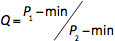, where P1 and P2 are the first and second highest correlation peaks, respectively, and min is the minimum value in the correlation plane. Q is a metric for assessing the quality of a vector. Q compares the highest correlation peak, which results in the best vector, to the common correlation background represented by the second highest correlation peak. Vectors with Q near 1 are an indication that the highest correlation peak is a false peak. Next, the median filter determines the median vector (u_median, v_median) of a group of vectors and the deviation of the neighboring vectors (u_rms, v_rms). The median filter rejects the middle vector (u,v) if it does not fit the following criteria: u_median - u_rms ≤ u ≤ u_median + u_rms and v_median - v_rms ≤ v ≤ v_median + v_rms. Additionally, it is possible to obtain groups of spurious vectors if a big overlap was specified in the velocity vector calculation. Therefore, it is possible to remove groups of vectors with less than a specified number of vectors. Once spurious vectors are removed, vector fill up may be used to fill up the empty spaces with interpolated vectors determined from non-zero neighboring vectors. Finally, applying the mask permanently will delete any vectors outside the mask.
10. Assess the quality of the results: a) Do the results make physical sense? (i.e. slower velocities near the boundary, increasing velocities with increasing distance from the wall; the direction of the vectors follow the general direction of the flow, etc.); b) The resulting vector field is largely composed of first choice vectors (indicated by the PIV processing software). Typically it is recommended that the fraction of first choice vectors be higher than 95%. A broader range of post processing steps is described in the literature, e.g. ^1,2.

Results

A photo of the set-up is shown in Figure 1. Raw particle images of a 32 x 32 pixel interrogation window near the wall from two consecutively captured images are shown in Figure 2. The particles in Figure 2a are displaced 2-3 pixels to the right in Figure 2b and satisfy the "one-quarter rule," which states that in-plane and out-of-plane particle displacements should not exceed ¼ of the interrogation window size. Additionally, the particle density per interrogation window should be roughly 8-10 particles since PIV correlation algorithms track groups of particles. However, the seeding density in near-wall PIV investigations is often on the order of 1-3 particles. Thus, special algorithms should be used to address studies with lower seeding density, such as particle tracking velocimetry (PTV) algorithms which track individual particles ^1,2,4-6. A time-averaged correlation approach ^7,8 may also be used to address low seeding density issues but this generally results in the loss of temporal resolution. Additionally, imaging near walls is impacted by bright laser reflections that may adversely affect PIV correlations and produce false vectors. These bright reflections also limit the position of the first valid velocity vector in the wall normal direction. Pre-processing the raw particle images is necessary to reduce the impact of background noise from sources such as laser reflections. In this demonstration the first valid vector was located 23 μm from the wall.

After raw particle images are processed using the PIV correlation algorithms, the quality and validity of the resulting velocity vector fields should be assessed. Spurious vectors are unavoidable in the raw vector fields but there are a few distinguishing characteristics. Incorrect vectors are common near surfaces, at the edges of the light sheet, and at the edges of a flow. In addition, the magnitude and direction of invalid vectors differ significantly from neighboring vectors and will not make physical sense. In the case of this boundary layer flow example, the valid velocity vectors should point from left to right as the particle displacements from Figure 2 indicate. Additionally, the velocities should decrease near the wall due to the no-slip condition ⁹. The instantaneous velocity fields shown in Figure 3 fit both of these physical criteria. Another useful metric to assess the validity of PIV results is to determine the vector choice of each vector in the velocity vector field. In general, the vector field should consist of >= 95% first choice vectors, i.e. those that required no post-processing, so that robust post-processing algorithms may be used to detect and replace spurious vectors without producing considerable artifacts ². The instantaneous vector fields shown in Figure 3 are composed entirely of 1st choice vectors.

The significance of high-speed, or cinematographic, PIV measurements becomes evident from an inspection of a time sequence of flow images. Instantaneous velocity (V_i) and velocity fluctuation (V') vector fields at the beginning, middle, and end of the recording sequence are shown in Figure 3. Using a Reynolds decomposition, V_i is the sum of the averaged velocity field () and V' ¹⁰. For this experiment, was determined by temporally averaging all images in the sequence. The instantaneous vector fields throughout the recording sequence are very similar and show the flow moving from the left to the right. These results also indicate that the flow is predominantly in the horizontal direction since the horizontal velocity component (u) is much larger than the vertical velocity component (v). The fluctuation vector fields also indicate that the horizontal velocity fluctuations (u') are larger than the vertical velocity fluctuations (V'). However, the fluctuations also indicate that the flow is slowing down since u' reverses its direction throughout the recording sequence.

The time-averaged and instantaneous u - profiles at several different times throughout the recording sequence are shown in Figure 4 and verify that the flow is slowing down over time. The u - profiles were determined by averaging four adjacent vector columns together to improve the statistical significance of the results close to the wall. The procedure was used in previous work ^6,8. The error bars indicate twice the standard deviation of the four adjacent vector columns. The largest error bar occurs near the surface of the plate and reaffirms the difficulty of using PIV correlation algorithms for areas of low seeding density. Several analysis algorithms are designed to address low seeding density such as PTV ^5,6 and time-averaged correlation approaches ^7,8.

Figure 1. Benchtop assembly.

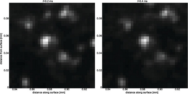
Figure 2. Particle images in a 32 x 32 pixel interrogation near the wall at a) t = 0.2 msec and b) t = 0.4 msec. The physical dimensions of the interrogation window are 96 x 96 μm².

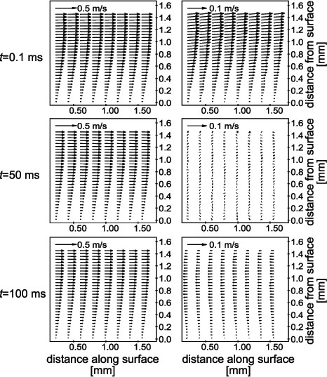
Figure 3. On the left: instantaneous (V_i), and on the right: fluctuation (V') velocity fields at the beginning, middle, and end of the recording sequence. Vector fields are composed entirely of first-choice vectors. A smaller subset of the vector fields is shown for clarity. The V_i fields indicate flow moving from left to right while V' reverse direction. Please note that only every fourth vector column in the horizontal direction is shown for clarity. Additionally, the velocity scale between the V_i and V' fields is different as indicated in the top left corner of each image.

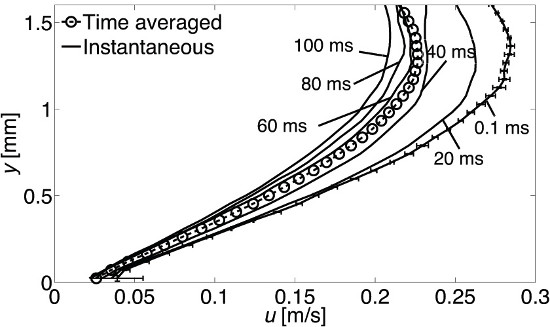
Figure 4. Horizontal velocity (u) profiles at different times throughout the flow. Time-averaged u - profile is shown with circles. Error bars shown on t = 0.1 msec profile are representative of error bars for all other times. The time history of the u - profiles shows a decrease in the flow over time.

Discussion

As with any optical flow measurement technique, planning the setup of high-speed particle image velocimetry (PIV) requires assessment of constraints and the evaluation of best compromises for the measurement task at hand. The selection of image magnification, frame rate, laser sheet properties, and analysis algorithms depend on details of the flow under study. If need be, exploratory measurements must be conducted to identify parameter settings for high fidelity measurements.

This article describes the general procedure and some sample results for high-speed PIV to study the boundary layer of a flow along a flat plate. A sequence of 500 images was recorded at 5 kHz. A long-distance microscope was used to achieve a 2.4 x 1.8 mm² field-of-view located at the plate surface. High quality illumination of the seed oil droplets was achieved with a beam from a pulsed diode-pumped solid-state laser that was expanded into a light sheet using a beam homogenizer. The beam homogenizer contains a micro-lens array made up of small cylindrical lenses and an additional, integrated telescope. The micro-lens array expands the circular beam in the vertical direction by splitting the incoming beam into beamlets. Then the following telescope superimposes the beamlets to create a light sheet with an even light intensity distribution in the light sheet plane normal to the beam propagation. Images were processed using a PIV cross-correlation algorithm. It should be noted that a homogenized beam is helpful, especially when working near surfaces, but it is not crucial to the application described here.

The method outlined in this procedure enables non-intrusive high-resolution, high-speed investigations of flows using robust correlation algorithms. The key advantages of this high-resolution, high-speed measurement technique are high spatial and temporal resolution and the ability to identify and track the evolution of structures within the flow. Using these techniques, Alharbi ⁶ and Jainski et al. ⁸ have demonstrated the ability to visualize and track vortex structures within the boundary layer of an internal combustion engine. These key features enable investigations on the structure and dynamics of highly transient flows. Furthermore, PIV may be expanded beyond the two-dimensional, two-component (2D-2C) velocity fields (as described here) to resolve 3-components (3C) in a plane (stereo-PIV) and in a volume (tomographic PIV, scanning PIV, holographic PIV). Additionally, PIV may be implemented with other techniques such as planar laser-induced fluorescence (PLIF), filtered Rayleigh scattering (FRS), and thermographic phosphors to achieve simultaneous 2D measurements of velocity and other scalars (temperature, species concentration, equivalence ratios) ^11-14. These optical, laser-based methods can be directly applied to investigate mass and energy exchange processes in many applications, such as the near-wall flows in an internal combustion engine.

Materials

List of materials used in this article

Name	Company	Catalog Number	Comments
High-speed 532 nm Nd:YAG laser	Quantronix	Model: Hawk I
Long distance microscope ( QM-100)	Questar	Model: QM-100
High-speed CMOS camera (Phantom v7.3)	Vision Research	Model: Phantom v7.3
Atomizer (TSI 9306)	TSI	Model: 9306
Silicone oil	Dow Corning CST 510	CST 510 Fluid
Beam homogenizer	Fraunhofer		Custom made part
45 ° high-reflectivity (HR) 532 nm turning mirror	Laser Optik		Multiple suppliers
Aperture			Multiple suppliers
Calibration target			Custom made part
PIV recording and processing software	LaVision	Software: Da Vis
High-speed controller (HSC)	LaVision
Optical rail and carriers			Multiple suppliers
Laser beam blocks and traps			Multiple suppliers
Mounts for optical elements			Multiple suppliers
Translation stage	Newport
Metal tubing to create jet flow	McMaster-Carr		Multiple suppliers
Combination square and centering square			Multiple suppliers