Lesion Explorer: A Video-guided, Standardized Protocol for Accurate and Reliable MRI-derived Volumetrics in Alzheimer's Disease and Normal Elderly

Summary

Lesion Explorer (LE) is a semi-automatic, image-processing pipeline developed to obtain regional brain tissue and subcortical hyperintensity lesion volumetrics from structural MRI of Alzheimer's disease and normal elderly. To ensure a high level of accuracy and reliability, the following is a video-guided, standardized protocol for LE's manual procedures.

Abstract

Obtaining in vivo human brain tissue volumetrics from MRI is often complicated by various technical and biological issues. These challenges are exacerbated when significant brain atrophy and age-related white matter changes (e.g. Leukoaraiosis) are present. Lesion Explorer (LE) is an accurate and reliable neuroimaging pipeline specifically developed to address such issues commonly observed on MRI of Alzheimer's disease and normal elderly. The pipeline is a complex set of semi-automatic procedures which has been previously validated in a series of internal and external reliability tests^1,2. However, LE's accuracy and reliability is highly dependent on properly trained manual operators to execute commands, identify distinct anatomical landmarks, and manually edit/verify various computer-generated segmentation outputs.

LE can be divided into 3 main components, each requiring a set of commands and manual operations: 1) Brain-Sizer, 2) SABRE, and 3) Lesion-Seg. Brain-Sizer's manual operations involve editing of the automatic skull-stripped total intracranial vault (TIV) extraction mask, designation of ventricular cerebrospinal fluid (vCSF), and removal of subtentorial structures. The SABRE component requires checking of image alignment along the anterior and posterior commissure (ACPC) plane, and identification of several anatomical landmarks required for regional parcellation. Finally, the Lesion-Seg component involves manual checking of the automatic lesion segmentation of subcortical hyperintensities (SH) for false positive errors.

While on-site training of the LE pipeline is preferable, readily available visual teaching tools with interactive training images are a viable alternative. Developed to ensure a high degree of accuracy and reliability, the following is a step-by-step, video-guided, standardized protocol for LE's manual procedures.

Introduction

Brain image analysis is an emerging field of neuroscience requiring skilled operators with a high degree of computational and neuroanatomical competency. In order to obtain quantitative information from magnetic resonance imaging (MRI), a trained operator is often required to implement, monitor, and edit, computer-generated imaging outputs generated from raw MRIs. While many ‘fully automatic' imaging tools are freely available via the internet, accuracy, and reliability is questionable when applied by a novice operator lacking knowledge, training and familiarity with the downloaded tool. Although on-site training is the most preferable teaching approach, the presentation of a video-guided, standardized protocol is a viable alternative, particularly if accompanied by a training set of images. Additionally, the training set of images may be used for quality control measures, such as an off-site inter-rater reliability test.

The challenges of developing an image processing pipeline, particularly when studying aging and Alzheimer's disease (AD), include a wide range of technical and biological issues. Although some technical issues are addressed with post-processing correction algorithms³, variability due to individual differences and pathological processes introduce more complex obstacles. Brain atrophy and ventricular enlargement can reduce the viability of registration warping and template-matching approaches. The presence of age-related white matter changes⁴ and small vessel disease^5,6, observed as subcortical hyperintensities (SH)^7,8, cystic fluid-filled lacunar-like infarcts^9,10, and dilated perivascular spaces^11,12, further complicate segmentation algorithms. In cases of significant white matter disease, a single T1 segmentation could result in overestimation of gray matter (GM)¹³, which can only be corrected with an additional segmentation using proton density (PD), T2-weighted (T2), or fluid-attenuated inversion recovery (FLAIR) imaging. In light of these challenges, the Lesion Explorer (LE) image processing pipeline implements a semi-automatic tri-feature (T1, PD, T2) approach, utilizing trained operators at particular stages when human intervention is preferable^1,2.

Brain extraction (or skull stripping) is typically one of the first operations performed in neuroimaging. Given this, the accuracy of the total intracranial vault (TIV) extraction process greatly influences subsequent operations further down the pipeline. Significant over-erosion, resulting in loss of brain, may lead to over-estimation of brain atrophy. Alternatively, significant under-erosion, resulting in inclusion of dura and other nonbrain matter, may lead to inflation of brain volumes. LE's Brain-Sizer component addresses many of these issues by using a tri-feature (T1, T2, and PD) approach to generate a TIV mask, which yields superior results compared to single-feature methods¹. Additionally, the automatically generated TIV mask is manually checked and edited using standardized protocol which identifies regions susceptible to skull stripping errors. After brain extraction, segmentation is performed on the skull-stripped T1, where each brain voxel is assigned to 1 of 3 labels: GM, white matter (WM), or cerebrospinal fluid (CSF). Segmentation is accomplished automatically using a robust curve-fitting algorithm applied to global and local intensity histograms; a technique developed to address intensity nonuniformity artifact and a decreased separation between GM and WM intensity amplitude in AD cases¹⁴.

The Brain-Sizer component also includes procedures for manual designation of ventricles and removal of subtentorial structures. Segmentation of ventricular CSF (vCSF) is particularly important as ventricle size is a commonly used biomarker for AD dementia¹⁵. Additionally, delineation of ventricles and choroid plexus is imperative for proper identification of periventricular hyperintensities (pvSH), which are believed to reflect a form of small vessel disease characterized by venous collagenosis^5,16,17. Using T1 for reference, manual relabeling of CSF voxels to vCSF is accomplished with manual floodfill operations on the segmented image. Typically, the lateral ventricles are easier to differentiate from sulcal CSF. For this reason, it is recommended to begin floodfilling in axial view, starting from superior slices and moving inferiorly. The medial parts of the ventricular system, particularly the 3^rd ventricle, is more difficult to delineate and is given special anatomy-based rules which are outlined in the manual. Brain-Sizer's final step includes removal of the brain stem, cerebellum, and other subtentorial structures, using manual tracing procedures described in an additional set of anatomy-based standardized protocols.

The Semi-Automated Brain Region Extraction (SABRE) component is the pipeline's parcellation procedure. This stage requires trained operators to identify the following anatomical landmarks: anterior and posterior commissure (AC, PC); posterior brain edge; central canal; mid-sagittal plane; preoccipital notch; occipito-parietal sulcus; central sulcus, and; Sylvian fissure. Based on these landmark coordinates, a Talairach-like¹⁸ grid is automatically generated and regional parcellation is accomplished¹⁹. Landmarks are easily identified on ACPC aligned images, which are generated automatically and manually checked prior to SABRE landmarking procedures.

The Lesion-Seg component is the final stage of the pipeline where SH identification and quantification is accomplished. The initial automatic SH segmentation implements a complex algorithm which includes PD/T2-based SH segmentation, fuzzy c-means masking, and ventricular dilatation. These operations result in an automatically generated lesion segmentation mask that is manually checked and edited for false positives and other errors. As hyperintense signal on MRI may result from nonpathological sources (e.g. motion artifact, normal biology), proper training is required for accurate identification of relevant SH.

The final result of the LE pipeline is a comprehensive volumetric profile containing 8 different tissue and lesion volumetrics which are parcellated into 26 SABRE brain regions. To obtain an individual operator's inter-rater reliability test off-site, it is recommended to execute the full LE pipeline on the training set provided with the software (http://sabre.brainlab.ca). Using the volumetric results, inter-class correlation coefficient (ICC)²⁰ statistics can be calculated for each tissue class (GM/WM/CSF) in each SABRE region. Using the segmentation images, Similarity Index (SI)²¹ statistics can be calculated to evaluate the degree of spatial congruence. Additionally, intra-rater reliability can be assessed on the same operator's results, after a brief period of time has passed between the operator's 1^st and 2^nd segmentation edits. Provided that the off-site operator adheres to the file naming conventions outlined in the LE manual, reliability statistics can be calculated off-site using most basic statistical software packages. Given these quality control and video-guided standardized protocol, off-site operators can have greater confidence that the LE pipeline is applied accurately and reliably.

Protocol

1. Brain-Sizer Component

1.1 Total Intracranial Vault Extraction (TIV-E)

1. Open ITK-SNAP_sb, load T1 Click: File -> Open grayscale image -> Browse -> go to directory, Click -> Image -> Open -> Next -> Finish.
2. Click plus sign next to axial view to enlarge.
3. Turn off (or on) crosshairs with 'x' key.
4. Right click and drag mouse upwards to enlarge brain in window until it fits without small box appearing in bottom left corner.
5. Adjust intensity by clicking: Tools -> Image Contrast, then drag middle point up and slightly left until the image brightens to the appropriate level, Close.
6. Load TIV-E overlay by clicking: Segmentation -> Load from image -> Browse -> Select TIVauto -> Open -> Next -> Finish.
7. Begin editing TIVauto…
8. Click Paintbrush tool -> Select round -> Adjust size as necessary.
9. To add in / recapture brain that TIVauto has not accounted for, select 'Active drawing label' as 'Label 1', and 'Draw over' as 'All Labels'.
10. To recapture colored TIV areas, or CAREFULLY recapture noncolored areas use paintbrush to repaint the TIV mask.
11. To undo a painting brush stroke, use <CTRL+Z> or click 'Undo' (on left).
12. Toggle TIVauto on/off by pressing 's' to verify that brain tissue is appropriately captured.
13. To remove/delete TIVauto mask if it over-captures nonbrain tissue right click using "paintbrush tool".
14. Use paintbrush and left click to repaint the TIVauto mask.
15. Check each and every slice carefully to make sure only brain tissue is Label 1 (green) and all nonbrain tissue is some label other than 1 (or not colored at all).
16. Recapture TIV as appropriate, and delete TIV as appropriate.
17. For superior slices make sure everything beneath the dura is kept to account for CSF.
18. If it is difficult to paint, use the closed polygon tool: Left Click to add points to the polygon and Right Click to close it such that everything contained within the polygon is what is being modified, then click "Accept" at the bottom, or if the tracing is incorrect, click "Delete". Polygon changes can be undone by clicking undo or <CTRL+z>. See Figure 1.
19. When satisfied with TIV modifications click: Segmentation -> Save as image -> and modify file name ending from "TIVauto" to TIVedit" to indicate that it is 'Done', then click 'Save' (e.g. <name>_TIVedit).

1.2 Ventricular Reassignment

1. Load the T1_IHC.
2. Adjust the intensity.
3. Turn off the crosshairs (x).
4. Select only the axial image to view by clicking the plus symbol next to the axial window.
5. Zoom in (right click and drag).
6. Load the <name>_seg image over the T1 by selecting segmentation -> Load from image -> Browse -> <name>_seg -> Next -> Finish.
7. Adjust the drawing labels to the appropriate colors, through label editor.
8. Change the colors such that 5 is purple, 7 is magenta, and 3 & 4 are something easily distinguishable from the rest (e.g. Figure 2 shows 3=WM change to blue, and 4=GM change to yellow). Note: colors are arbitrary.
9. Reassign vCSF by using the floodfill tool. See Figure 2.
10. Go up slices through the brain to determine the most superior slice with ventricle and begin there.
11. Click the floodfill tool, Select 'Active drawing label' =7 and 'Draw over' =5.
12. Toggle back and forth between 'Floodfilling' and Drawing Limits by pressing the SPACEBAR. Limits are used to prevent the floodfill from filling certain areas of the ventricle that are considered periventricular black holes or part of white matter hyperintensities.
13. When floodfilling, a green arrow tip is visible, and when ready to draw a limit, a red arrow tip will be visible.
14. To fill, simply left click. Move down a slice, and repeat as necessary. Use limits as required to prevent floodfilling of nonventricle regions.
15. If floodfilling operations are incorrect, simply click 'Undo", or reverse the 'Active drawing label' and 'Draw over' colors.
16. Fill every voxel that connects to ventricle, knowing what not to fill is just as important as knowing what to fill.
17. Continue moving down until the 3^rd ventricle opens into the quadrigeminal cistern and draw a limit at the posterior edge of the quadrigeminal cistern until the posterior commissure separates the third ventricle from the quadrigeminal cistern.
18. A limit is necessary if the posterior commissure is not fully visible and does not create an enclosed space. Once the posterior commissure creates an enclosed space, discontinue relabelling the quadrigeminal cistern.
19. Limits may also be necessary if the anterior commissure does not enclose the 3^rd ventricle.
20. Stop filling the 3^rd ventricle once the cerebral peduncles are clearly visible on T1, and the central canal is round.
21. Limits may also be necessary with the anterior portion of the lateral ventricles around the brainstem, if they appear to connect to the sulcal CSF.
22. Use the T1 as a guide on what to fill and what not to fill for temporal lobe lateral ventricles (Toggle segmentation on and off with 's' key).
23. When finished, save the segmentation as '<name>_seg_vcsf' by clicking: Segmentation -> Save as image- > and then add _vcsf after <name>_seg -> Save.

1.3 Removal of Brain Stem, Cerebellum, and Subtentorial Structures

1. Select 'Polygon tool' from top left menu.
2. Toggle segmentation off.
3. Scroll to first slice on which cerebellum begins (if brainstem separates before cerebellum begins, see rule exceptions).
4. Select 'Active drawing label' = 'Clear Label' and 'Draw over' = 'All Labels'.
5. These active drawing labels essentially DELETES data from the segmentation image, so exercise caution. Undo (CTRL+Z) still works, but only for a limited number of steps back.
6. Left click to draw a polygon over the dura surrounding the cerebellum, and along the base of the brainstem across the colliculi. Right click to close polygon.
7. Click 'Accept' to 'Delete' that area of the segmentation, which will now show the T1 beneath indicating it is no longer included in the segmentation.
8. Go to the next slice down and repeat. Always do the tracings on the T1, never on the seg.
9. Once the cerebral peduncles separate, begin also removing the brainstem and spinal cord.
10. At the anterior aspect, trace directly across the gap. Once there is a clear dural line at the anterior orbitofrontal end (generally beneath the level of the pituitary, start tracing an arch out along that dura line).
11. Once the occipital lobe separates from the temporal lobe, ensure that the tracing exits from the center, to remove any remaining 'junk' in this region. See Figure 3.
12. At some point, draw the polygons so that they only keep what is required, instead of removing what is unnecessary, using the 'draw inverted' option (while referring to the seg to assist in the tracing).
13. If only temporal lobes remain, simply draw a large poly around the cerebellum and remove that.
14. If it is certain that the polygon will only contain cerebellum on a subsequent slice below, use the "paste" button to paste on the previous tracing and use that to delete the cerebellum.
15. Once the cerebellum is all that remains in the image, paste the large tracing down each slice and "accept" to delete it until there is no more cerebellum in the image.
16. Now scroll up through the image slice by slice to verify that the ONLY portions of the segmentation that remain are supratentorial.
17. When finished, save the segmentation as '<name>_seg_vcsf_st' by clicking: Segmentation -> Save as image- > and then add '_vcsf_st' after '_seg' -> Save.

2. SABRE Component

2.1 ACPC Alignment

1. Open ITK-SNAP_sb.
2. Load 'T1_IHCpre_iso' as described in Brain-Sizer manual.
3. Adjust intensity as described in Brain-Sizer manual.
4. Select the 'Navigation tool' from the top left menu.
5. Then click on the 'ACPC alignment tool'.
6. Load "T1_IHCpre_toACPC.mat" matrix file using load option in bottom left hand corner.
7. Zoom in to the image by right-clicking on the axial view and dragging the mouse upwards.
8. Change the position of the brain in the window (separate from zooming) by left-clicking on the image and moving the mouse around to better center the zoomed view. Also adjust the sagittal and coronal views. Make sure the sagittal view is close to mid-sagittal.
9. Click on 'ACPC tool' button.
10. Change the increment to 1.
11. Check Pitch, Roll and Yaw determined by T1_IHCpre_toACPC.mat matrix file, modify if necessary.
12. To find the ACPC plane, it is likely necessary to zoom in closely using the navigation tool. At any point, switch back and forth between the navigation tool and the ACPC tool (to adjust the view), and the ACPC tool will keep the position and return it to the previous position. When switching between these views, the image will change back and forth, but this is normal.
13. By using the pitch up/down and elevate up/down, adjust the axial view so that the AC is at its thickest (a nice u-shape of white matter fibers), and the PC straight across, which should end up forming a nice 'key hole' shape.
14. The AC-PC should also be visible with the crosshairs passing directly through both the AC and PC on the mid-sagittal view.
15. Do not adjust the pitch any further once this slice has been determined. However, the 'elevate' function can be used to move up and down through the image without losing the ACPC slice.
16. Now adjust the roll by balancing the eyeballs in the axial view. Readjust the view using the navigation tool to bring the eyeballs in to the field of view, then switch back to the 'ACPC' tool.
17. Use 'Roll' left or right to make sure that the eyeballs look evenly balanced (same size on both sides) while scrolling through the image one slice at a time using 'Elevate', making sure to adjust the roll as necessary. See Figure 4.
18. Once satisfied with the balance, Do not adjust 'Roll' any further.
19. Now move to a slice above the ventricles and corpus callosum in axial view (by using 'Elevate', or clicking the crosshairs at that level using 'Navigation') and place the crosshairs close to the center of the brain in axial view.
20. Adjust 'Yaw' by making sure that the vertical crosshair passes directly (or as close as possible) through the mid-sagittal plane in the axial view. Sometimes it may be difficult to get the plane to perfectly line up due to natural curvature of the brain at the poles - create the best fit possible.
21. Once satisfied with the position, Do not adjust 'Yaw' any further.
22. Now place crosshairs such that axial slice is just above the ventricles.
23. This should be approximately where it was from the previous step.
24. Now click: Save (make sure the filename is 'T1_IHCpre_toACPC.mat') -> OK.
25. NOTE: If "T1_IHCpre_toACPC.mat" matrix file does not require modification simply close without saving.
26. If changes were made to the matrix file, save over "T1_IHCpre_toACPC.mat" matrix file or save a new matrix file and delete the "T1_IHCpre_toACPC.mat" matrix file. The next command will not work correctly if there is more than 1 matrix file.

2.2 SABRE Landmark Identification

Part 1 - Grid File Coordinates

1. Load in '<name>__T1_IHC_inACPC'.
2. Adjust intensity.
3. Turn off crosshairs (x).
4. Zoom in to the image until it fills each window (right click and drag with crosshairs tool).
5. Adjust center of axial view if necessary, with navigation tool (may need to do several times during procedure).
6. Click on '2D-sabre land-marking' tool.
7. In axial view, scroll up through the images/brain until you find the ACPC slice.
8. Click the 'AC' radio button on the left to select that landmark to define, then click on the AC in the axial view.
9. A small dot will appear on the spot you clicked, and the associated landmark coordinate will now appear next to the 'AC' button on the left.
10. If the placement is not desirable, click again and the point will update (this applies to any point during the creation of the grid file).
11. Click the 'PC' radio button on the left and then click on the PC on the axial image.
12. Click the 'PE' radio button to define the posterior edge of the brain on that slice, and then click on the most posterior part of the brain, either on the left or the right - this fills in values for 'coronal slice' which will be used momentarily. See Figure 5.
13. Click the 'CA' radio button to define the central canal. Scroll down 10 slices from the current axial view and click on the center of the central canal. This fills in the value for 'sagittal slice' which will be used now as a starting point for which to find the mid-sagittal plane.
14. Click on the 'M' radio button to define the mid-sagittal plane.
15. In sagittal view, scroll left and right a few slices to determine which slice has the least amount of brain and the maximal amount of falx cerebri. It should be within 2 or 3 slices of the value determined from the central canal point.
16. Click anywhere on the mid-sagittal slice and that slice number will be entered on the left next to 'M'.
17. Click on the 'LPRON' radio button to define the left preoccipital notch. In coronal view, scroll to the slice indicated next to 'coronal slice'.
18. Click on the most inferior part of the brain for the left hemisphere, which appears on the RIGHT side of the image (radiological convention).
19. Click on the 'RPRON' radio button to define the right hemisphere, and click on the most inferior part of the LEFT side of the image (radiological convention).
20. The values next to LPRON and RPRON should now be filled, and should be within a few points of each other.
21. The grid file is now ready to be saved. Click: Save -> _T1_IHC_inACPC_lobgrid.txt.

Part 2 - Object Map Creation

22. After grid file creation, the next stage is the creation of the first 4 tracings of the object map. All of these 4 tracings are performed in the sagittal plane. The slices for tracing are predetermined and based on the midline slice selected in the previous stages.
23. Click on the 'RSC' radio button to define the right superior central sulcus. Go to the slice indicated next to 'Right Sagittal slice'. The left and right sagittal slices on which the tracings will be made: 7 slices peri-sagitally from the midline on each side.
24. Click a point directly above the center of the central sulcus, in the dura. The central sulcus on this slice generally appears as a small indentation, and is most commonly the first sulcus anterior to the marginal (ascending) branch of the cingulate sulcus. Scroll left or right to confirm the location of the landmark, but the tracing must always be made on the proper sagittal slice. Reclicking will relocate the landmark.
25. Click on the 'ROP' radio button to define the right occipito-parietal sulcus. This sulcus/tracing runs from the dura to the tentorium cerebelli.
26. A spline tool will now allow sulcus tracing. Left click to create new points along it, and right click to lock it and then click accept. Modifications or 'undo' functions can not be performed if there are errors made DURING the tracing. However, once the 'right-clicking' action is performed to complete the tracing, select 'Delete' to redo the tracing.
27. When the tracing is complete, select 'Accept' to lock it in.
28. Do the same for the left side at the appropriate slice, defining 'LSC' and 'LOP'.
29. Click: Save (under object map) -> _T1_IHC_inACPC_lobtrace.obj.

Part 3 - Surface Rendered Tracings

31. Unload previous images (or close and open ITK-SNAP_sb again) and load in <name>_T1_IHC_erode_inACPC image.
32. Click on the 3D SABRE landmarking tool (the window should enlarge to only show 1 pane).
33. Click 'LEFT' under 3D Viewpoint to show the left rendered view (in radiological convention, whereby left and right are reversed, so it will appear as though it is the right hemisphere).
34. Load in object tracing from previous step by clicking: Load -> Select '<name>_T1_IHC_inACPC_lobtrace.obj' (NOTE: a bug in the program automatically tries to anticipate loading the required file, but it incorrectly inputs 'erode' in the obj file name. Please select browse and then select the <name>_T1_IHC_inACPC_lobtrace.obj' to load. Otherwise an error message will be displayed, 'Error loading object map tracing: File cannot be opened for reading').
35. To adjust the quality of the render, click: 'Guess', to have the program guess at the best parameters to use.
36. Click 'LSF' radio button to prepare to trace the Left Sylvian Fissure.
37. Now click 'Landmark' button at the bottom of the 3D render window to begin landmarking/tracing (you can toggle this on and off with the "x" key).
38. Additional points to the tracing can be added when the 'Landmark' button is shaded green.
39. When 'Landmark' is unselected, any mouse input will rotate the brain to examine it from a different angle. WARNING: Only trace the landmarks while in straight 'LEFT' or 'RIGHT' orientation by reclicking on the left or right 3D Viewpoint buttons.
40. Zoom in to or out of the image by right clicking and dragging when 'Landmark' is unselected.
41. Each click will add a point to the line.
42. Begin tracing the Sylvian fissure from the superior to posterior end, at the point at which it bifurcates into small ascending and descending rami.
43. Continue tracing the Sylvian down the superior aspect of the temporal lobe until it trails off the end.
44. If an error is made, simply click the 'Undo' button to move backwards step by step (or press CTRL+Z).
45. Once satisfied with the tracing, click on 'Accept' to lock in the tracing. See Figure 5.
46. IMPORTANT: If redo is required for one of the tracings, first select the radio button (on the left) of the incorrect tracing. Then click 'SABRE3D' on the menu bar at the top and select 'Delete CURRENT Accepted Tracing'. If at some point all of your tracings require removal, click on 'Delete ALL accepted tracings' from this drop down menu.
47. Now click the 'LC' radio button to trace the Left Central Sulcus.
48. Start from the inferior end at the point of Sylvian fissure directly below the termination of the sulcus.
49. The line will only allow superior and posterior movement- meaning the program prevents placing points that are anterior to any previous point.
50. Finish tracing the sulcus at the superior end until it is difficult to follow the curvature of the brain.
51. Once complete, click 'Accept' to lock it in.
52. Now click on the 'RIGHT' button under '3D Viewpoint' and repeat the steps for the right Sylvian Fissure and Central Sulcus.
53. Remember to click on the 'RSF' radio button to trace the right Sylvian Fissure, and click on the 'RC' radio button to trace the right central sulcus, clicking 'Accept' after each tracing is complete.
54. Once all tracings are completed, click: Save -> Browse -> select '<name>_T1_IHC_erode_inACPC_lobtrace.obj'.
55. Close ITK-SNAP_sb.

3. Lesion-Seg Component

3.1 For Scans with PD/T2 (no FLAIR)

1. Open ITK-SNAP_sb, load <name>T1_IHC, <name>_PD_inT1­_IHC, <name>_T2_inT1_IHC, Click: File -> Open grayscale image -> Browse -> go to directory, Click -> Image -> Open -> Next -> Finish.
2. Click plus sign next to axial view to enlarge.
3. Turn off the crosshairs (x).
4. Zoom in (right click and drag).
5. Adjust intensity by clicking: Tools -> Image Contrast, then drag middle point up and slightly left until the image brightens to the appropriate level, Close.
6. Load lesion-seg on PD_inT1_IHC by clicking: Segmentation -> Load from image -> Browse -> Select <name>_LEauto -> Open -> Next -> Finish.
7. Adjust intensity of all 3 images as described in Brain-Sizer manual.
8. Click the paintbrush tool, Select 'Active drawing label' =2 and 'Draw over' =Visible labels.
9. Use T1, PD and T2 to inform decision about what to capture as lesion.
10. Use paintbrush tool to paint label 2 over label 1 to signify lesion (positives) (Toggle segmentation on and off with 's' key).
11. Use paintbrush tool to paint label 1 over label 2 to signify false positives. See Figure 6.
12. When satisfied with lesion-seg modifications click: Segmentation -> Save as image -> and modify file name by replacing "auto" with "edit" to the end of the file to indicate that it is 'Done', then click 'Save' (i.e. <name>_LEedit)

NOTE: Label 2 (default color is RED) is used to signify lesion.

3.2 For Scans with FLAIR Imaging

1. Open ITK-SNAP_sb, load <name>_FL_inT1_IHC Click: File -> Open grayscale image -> Browse -> go to directory, Click -> Image -> Open -> Next -> Finish.
2. Click plus sign next to axial view to enlarge.
3. Turn off the crosshairs (x).
4. Zoom in (right click and drag).
5. Adjust intensity by clicking: Tools -> Image Contrast, then drag middle point up and slightly left until the image brightens to the appropriate level, Close.
6. Load lesion-seg on FL_inT1_IHC by clicking: Segmentation -> Load from image -> Browse -> Select <name>_FLEXauto -> Open -> Next -> Finish.
7. Adjust intensity as described in Brain-Sizer manual.
8. Click the paintbrush tool, Select 'Active drawing label' =2 and 'Draw over' =Visible labels.
9. Use FL (use T1, PD, T2 if necessary) to inform decision about what to capture as lesion.
10. Use paintbrush tool to paint label 2 over label 1 to signify lesion (positives) (Toggle segmentation on and off with 's' key).
11. Use paintbrush tool to paint label 1 over label 2 to signify false positives. See Figure 7.
12. When satisfied with lesion-seg modifications click: Segmentation -> Save as image -> and modify file name by changing "auto" to "edit" to indicate that it is 'Done', then click 'Save' (i.e. <name>_FLEXedit).

NOTE: Label 2 (default color is RED) is used to signify lesion.

Results

Inter-rater reliability can be assessed using several metrics. Using the training set provided online (http://sabre.brainlab.ca), the following steps are recommended to assess inter-rater reliability for each of the processing stages after completion of LE.

Brain-Sizer:
To assess inter-rater reliability of the brain extraction procedures, generate volumetrics for each TIV-E masks, _TIVedit, using the command. Enter these volumetrics into a statistical software package (e.g. SPSS), along with the TIVedit volumetrics provided for each of the training set (see Excel/csv file provided online) and calculate the inter-rater correlation coefficient (ICC). Whole brain volumetrics for in-house trained raters obtain reported ICC=0.99, p<0.0001 ^1,2. Additionally, evaluation of the spatial agreement for the TIV masking can be assessed using the SI²¹. MATLAB code is provided online to calculate SI values between two raters.

To assess ventricular reassignment, generate vCSF volumes using the command for each of the segmentation files with the vCSF voxels reassigned, i.e. _ seg_vcsf. The vCSF volume is the value beside row ‘7’ under the column titled ‘volume’. Using the same procedures to evaluate TIV inter-rater reliability, calculate ICC and SI for vCSF.

Removal of brain stem, cerebellum and subtentorial structures can be assessed similarly by running the command on _seg_vcsf_st. The volumes used for this segmentation mask are shown at the second last row titled ‘total count of nonzero voxels:’ under ‘volume’ (the last column on the right). Using the same procedures to evaluate TIV and vCSF, calculate ICC and SI for this masking procedure using the volumetrics in the excel file provided and the _seg_vcsf_st files.

SABRE:
While Brain-Sizer’s manual procedures can easily be assessed using standard metrics, ACPC alignment is slightly more difficult. For this reason, matrix files are provided to compare visually for training of off-site operators. After completion of ACPC alignment, open a new ITK-SNAP_sb window, load the T1 image, then load the matrix for the training case provided online, _T1_IHCpre_toACPC.mat, and visually compare the pitch, roll, yaw, and ACPC slice between the two images.

To evaluate SABRE landmarking procedures, run on the parcellated mask, _SABREparcel_inACPC for each training case. Enter the volumetrics for each region (3-28). SABRE region codes are provided online. Using the same procedures to evaluate TIV and vCSF, calculate ICC for each SABRE brain region. SABRE parcellated regional volumetrics for in-house trained raters obtain reported mean ICCs=0.98, p<0.01, with ICC values ranging from 0.91-0.99 ^1,2.

Lesion-Seg:
As this component is the final stage of the LE pipeline, reliability and accuracy will depend on the prior stages.

Inter-rater reliability of SH segmentation is accomplished using regional ICC of SH volumes and spatial agreement of the SH masks. To evaluate regional SH volumes, run , entering both the lobmask file in T1-acquisition space, _SABREparcel and the final edited lesion segmentation file, _LEedit. Using the same procedures to evaluate SABRE volumetrics, calculate ICC for lesion volumes within each SABRE brain region. Using the same procedures to evaluate spatial agreement of the TIV masking process, calculate SI for the final edited lesion masks, _LEedit (or FLEXedit). The same reliability tests can be performed on both PD/T2-based segmentation and FLAIR-based segmentation.

	3D T1	PD/T2
Imaging Parameters	Axial Volume SAT (S1) SPGR	Axial Spin Echo FC VEMP VB (interleave)
Pulse Timing
TE (msec)	5	30/80
TR (msec)	35	3,000
Flip Angle (°)	35	90
TI (msec)	N/A	N/A
Scan Range
FOV (cm)	22	20
Slice thickness (mm)	1.2/0	3/0
No. Slices	124	62
Acquisition
Matrix size	256 x 192	256 x 192
Voxel size (mm)	0.86 x 0.86 x 1.4	0.78 x 0.78 x 3
NEX	1	0.5
Total Time (min)	11:00	12:00

Table 1. General Electric 1.5T Structural MRI Acquisition Parameters.

	3D T1	PD/T2	FLAIR
Imaging Parameters	Axial 3D FSPGR EDR IR Prep	Axial 2D FSE-XL, EDR, FAST, fat sat	Axial T2Flair, EDR, FAST
Pulse Timing
TE (ms)	3.2	11.1 / 90	140
TR (msec)	8.1	2,500	9,700
Flip Angle (°)	8°	90°	90°
TI (msec)	650	N/A	2,200
Scan Range
FOV (cm)	22	22	22
Slice thickness (mm)	1	3	3
No. Slices	186	48	48
Acquisition
Matrix size	256 x 192	256 x 192	256 x 192
Voxel size (mm)	0.86 x 0.86 x 1	0.86 x 0.86 x 3	0.86 x 0.86 x 3
NEX	1	1	1
Total Time (min)	7:20	6:10	7:20

Table 2. General Electric 3T Structural MRI Acquisition Parameters.

Figure 1. Axial T1 with unedited total intracranial vault (TIV) mask overlay (green). This is an example of the use of the closed polygon tool in ITK-SNAP_sb to remove nonbrain tissue as part of the manual editing procedure of the Brain-Sizer’s TIV extraction procedure.

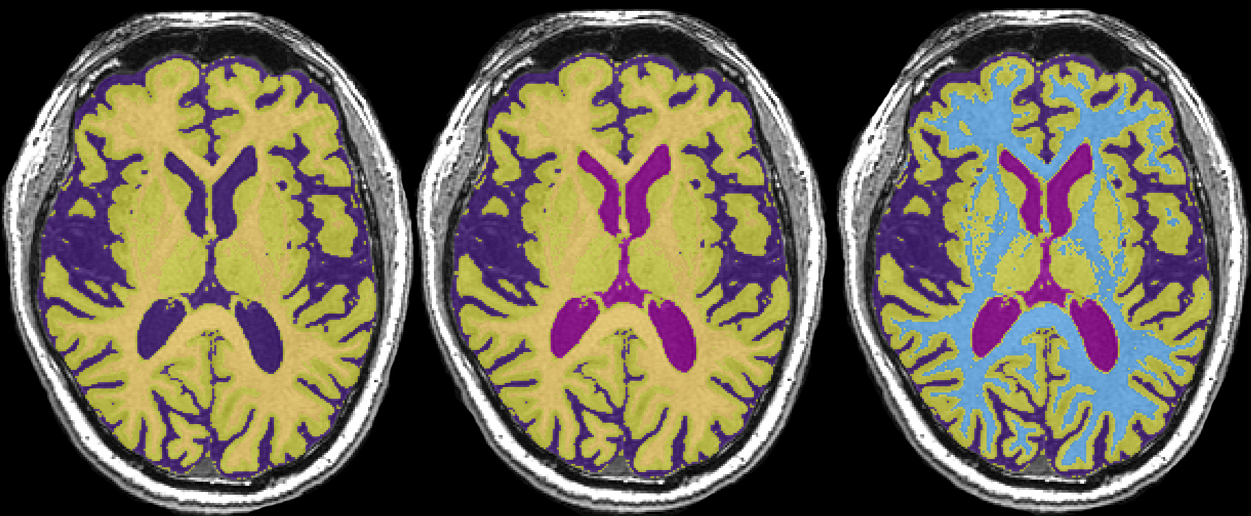
Figure 2. Axial T1 with tissue segmentation overlay. Note that label colors are arbitrary and can be modified using the Label tool. Left image shows default colors. Middle image shows how CSF (5=purple) is reassigned to vCSF (7=magenta). Right image shows how the WM color can be modified without changing the tissue class label, i.e. Label 3=WM remains but color can be modified to blue.

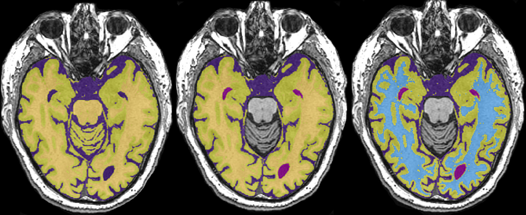
Figure 3. Axial T1 with tissue segmentation overlay (left image, GM=yellow, WM=orange, CSF =purple) (left). Depicted is an example of manual removal of subtentorial structures using the closed polygon tool in ITK-SNAP_sb (middle) and final tissue segmentation after removal (right). As in Figure 2, right image shows how the WM color can be modified without changing the tissue class label, i.e. Label 3=WM remains but color can be modified to blue.

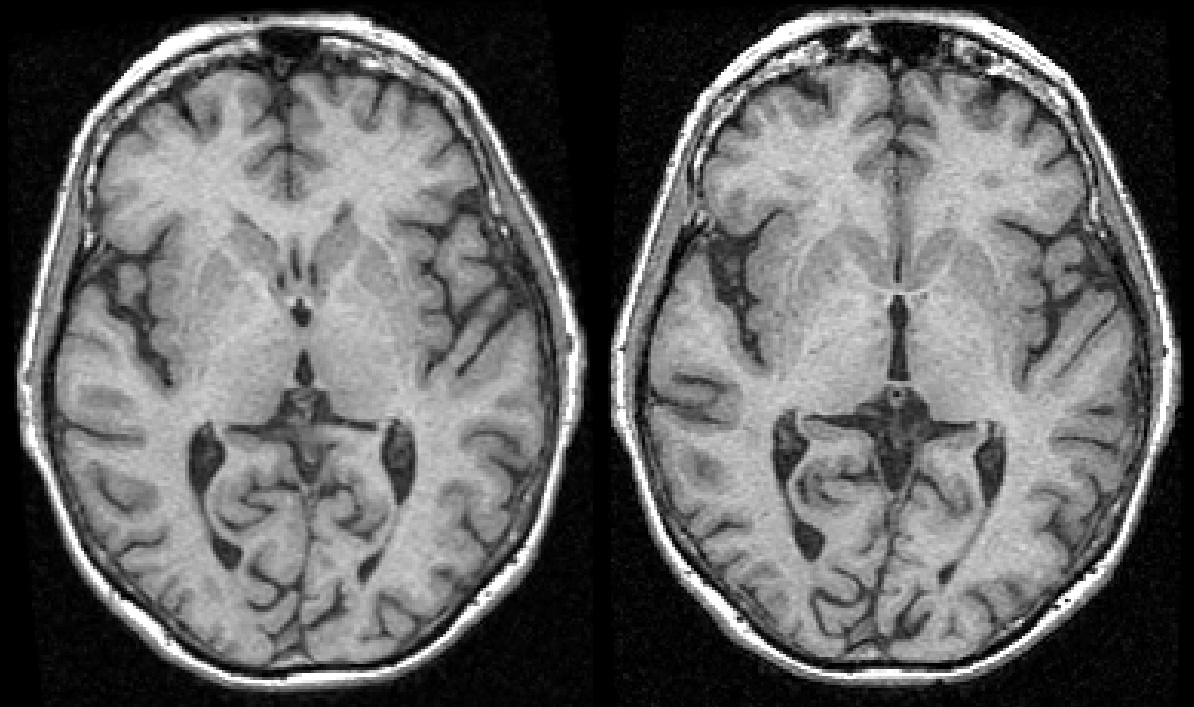
Figure 4. Axial T1 in acquisition space before (left), and after (right) AC-PC alignment is performed.

Figure 5. Two examples showing SABRE landmarking procedures. Axial AC-PC aligned T1 with AC (yellow), PC (blue), and posterior edge (pink) landmark placements (left). A 3D surface-rendered T1 (right) with Sylvian fissure (purple) and central sulcus (pink) delineation.

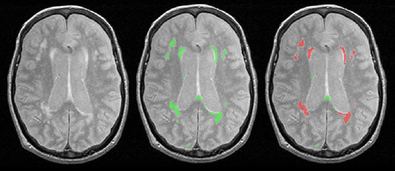
Figure 6. Axial PD (left) with automatically generated lesion overlay (center), and manually edited lesion (red) overlay (right).

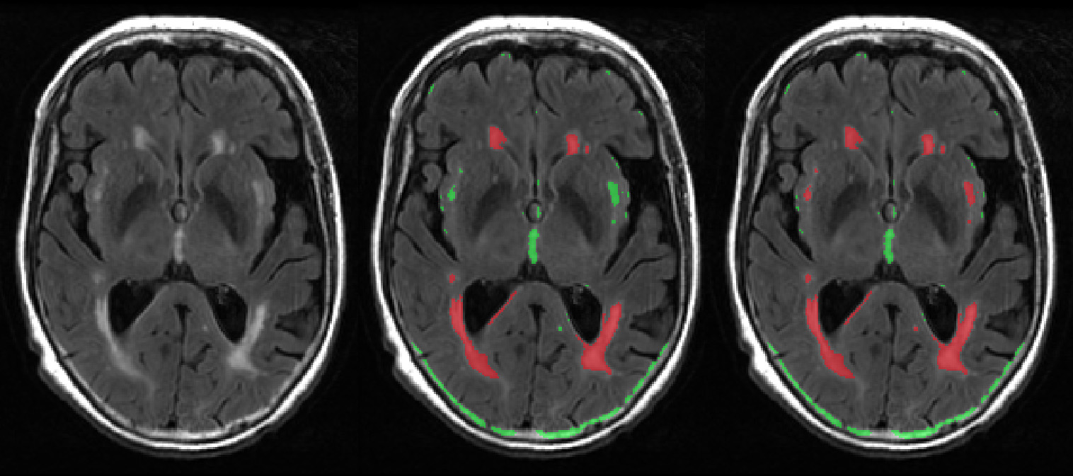
Figure 7. Axial FLAIR (left), with automatically generated lesion overlay (center), and manually edited lesion (red) overlay (right).

Discussion

The LE segmentation and parcellation procedure was developed specifically to obtain regional volumetrics from MRI of AD and normal elderly. While there are numerous fully automatic pipelines which apply complex computational algorithms to perform these operations, these tools tend to lack the individualized accuracy and precision that LE’s semi-automatic pipeline produces. The trade-off with semi-automatic processes are the resources required to properly train operators with the anatomical knowledge and computational skills needed to apply such a comprehensive pipeline. However, one of the primary benefits of an individualized imaging pipeline is the ability to obtain quantitative volumetrics from moderate to severe cases of neurodegeneration when automatic pipelines fail.

As the LE pipeline has been previously evaluated and applied to various elderly and demented populations^{1,2,13,14,19,22,23}, the main issues that are typically encountered by trained operators have been well-documented and are summarized below.

The manual checking and editing required with the Brain-Sizer component includes the TIV extraction masking procedure, vCSF reassignment and manual removal of the brain stem, cerebellum and other subtentorial structures. For brain extraction, the automatic TIV output is generally a decent mask provided that the original PD/T2 images are good quality. However, due to the relative intensity values of vascular and nerve tissue medial to the inferior temporal poles, proximal to the carotid arteries, this region typically requires some editing. Additionally, mucous in the nasal cavity tends to affect regional intensity histograms, skewing intensity cut-offs values in the anterior frontal regions, which tend to require additional manual editing of the automatic TIVauto mask. Finally, additional manual editing is typically required in the most superior regions, where global atrophy tends to result in an increase in the volume of subarachnoid CSF just below the dura mater. Alternatively, atrophy associated with ventricular enlargement tends to minimize operator interventions required with vCSF reassignment. Another benefit of having a tri-feature coregistration approach is the ability to identify cystic fluid-filled infarcts proximal to the ventricles, potentially due to periventricular venous vasculopathy^5,24-26, which are identifiable due to their relative intensity on PD and T1 (hyperintense on PD, hypointense on T1). These hypointensities can be delineated from vCSF using manual limits drawn in ITK-SNAP_sb prior to floodfilling operations. Since vCSF reassignment is performed in T1-acquisition space, in cases where alignment deviates far from the ACPC plane, a limit may be required for the 3^rd ventricle and the quadrigeminal cistern, if the PC is not fully visible. Although the tentorium is a relatively easy structure to differentiate, several anatomy-based rules assist in guiding manual removal of the brain stem and subtentorial structures, particularly when locating the separation of the cerebral peduncles from the medial temporal lobe.

SABRE landmarking is a stereotaxic-based procedure performed in standard ACPC aligned images, allowing for moderately predictable localization of particular anatomical landmarks. Exceptions to this are cases with extreme atrophy and normal variability due to individual differences in neuroanatomy. Brain atrophy results in an overall loss of parenchyma, increasing CSF along the midline surrounding the falx cerebri, which increases the difficulty of choosing appropriate points to place landmarks. Rule-based protocols are required, identifying cases where exceptions to the general rule are required. Normal variations in anatomy, particularly in the relative location of the central sulcus and the parieto-occipital sulcus, also increase the difficulty of manual delineation of these structures. However, the graphical user interface used by SABRE allows for real-time rotation of surface rendered images, which significantly assists in the decision-making process for visualization of these particular landmarks. Finally, some rule-based protocol have been integrated programmatically into the software to prevent operator violation e.g. central sulcus delineation is forced to move posteriorly (line tracing is prevented from going back onto itself).

The Lesion-Seg component’s manual checking procedure requires expertise in visual identification of relevant hyperintensities, a visual perception skill that is only acquired after exposure to scans with varying degrees of SH. False-positive minimization algorithms assist with the removal of most errors in the initial segmentation. However, differentiation between dilated perivascular spaces (Virchow-Robin spaces: VRS) in the lentiform nucleus and relevant SH in the external capsule, claustrum, extreme capsule, and subinsular regions can be difficult. This is particularly difficult in cases with VRS in the basal ganglia. A recent paper outlining STandards for ReportIng Vascular changes on nEuroimaging (STRIVE), recommended a size criterion to differentiate VRS from lacunes, and describe VRS to be more linear and CSF intensity on MRI. To address these issues with VRS identification, LE has adopted: a) an anatomy-based rule which prevents operators from selecting any hyperintensity that falls within the lentiform nucleus, b) a size criterion to exclude hyperintensities less than 5mm in diameter, and c) a relative intensity rule for additional exclusion due to the relative CSF intensity on PD, T2 and T1²⁷. Additionally, normal hyperintense signal can be found along the midline and falx cerebri, particularly on FLAIR imaging, which can be difficult to differentiate between relevant SH along the corpus callosum. In cases of such overlap, anatomy-based rules are implemented where only SH which extend out into the periventricular regions are accepted.

In conclusion, it is important to appreciate that this written component is meant to supplement a video-guided, standardized protocol publication in JoVE (http://www.jove.com). While traditional static figures assist in explaining some concepts, video-based tutorials are more efficient at communicating the complex methodological processes involved with a comprehensive neuroimaging pipeline such as Lesion Explorer.

Materials

List of materials used in this article

Name	Company	Catalog Number	Comments
Magnetic resonance imaging machine (1.5 Tesla)	General Electric		See Table 1 for acquisition parameters
Magnetic resonance imaging machine (3 Tesla)	General Electric		See Table 2 for acquisition parameters

References

- Ramirez, J., Gibson, E., Quddus, A., Lobaugh, N. J., Feinstein, A., Levine, B., Scott, C. J., Levy-Cooperman, N., Gao, F. Q., Black, S. E. Lesion Explorer: A comprehensive segmentation and parcellation package to obtain regional volumetrics for subcortical hyperintensities and intracranial tissue. Neuroimage. 54 (2), 963-973 (2011).
- Ramirez, J., Scott, C. J., Black, S. E. A short-term scan-rescan reliability test measuring brain tissue and subcortical hyperintensity volumetrics obtained using the lesion explorer structural MRI processing pipeline. Brain Topogr. 26 (1), 35-38 (2013).
- Sled, J. G., Zijdenbos, A. P., Evans, A. C. A nonparametric method for automatic correction of intensity nonuniformity in MRI data. IEEE Trans. Med. Imaging. 17 (1), 87-97 (1998).
- Wahlund, L. O., Barkhof, F., Fazekas, F., Bronge, L., Augustin, M., Sjogren, M., Wallin, A., Ader, H., Leys, D., Pantoni, L., Pasquier, F., Erkinjuntti, T., Scheltens, P. A new rating scale for age-related white matter changes applicable to MRI and. 32 (6), 1318-1322 (2001).
- Pantoni, L. Cerebral small vessel disease: from pathogenesis and clinical characteristics to therapeutic challenges. Lancet Neurol. 9 (7), 689-701 (2010).
- Black, S. E., Gao, F. Q., Bilbao, J. Understanding white matter disease: Imaging-pathological correlations in vascular cognitive impairment. Stroke. 40, (2009).
- Arch Neurol, 44, 21-23 (1987).
- Carmichael, O., Schwarz, C., Drucker, D., Fletcher, E., Harvey, D., Beckett, L., Jack, C. R., Weiner, M., Decarli, C. Longitudinal changes in white matter disease and cognition in the first year of the Alzheimer disease neuroimaging initiative. Arch. Neurol. 67 (11), 1370-1378 (2010).
- Wardlaw, J. M. What is a lacune. Stroke. 39 (11), 2921-2922 (2008).
- Potter, G. M., Doubal, F. N., Jackson, C. A., Chappell, F. M., Sudlow, C. L., Dennis, M. S., Wardlaw, J. M. Counting cavitating lacunes underestimates the burden of lacunar infarction. Stroke. 41 (2), 267-272 (2010).
- Barkhof, F. Enlarged Virchow-Robin spaces: do they matter. J. Neurol. Neurosurg. Psychiatry. 75 (11), 1516-1517 (2004).
- Zhu, Y. C., Dufouil, C., Soumare, A., Mazoyer, B., Chabriat, H. Tzourio C. High degree of dilated Virchow-Robin spaces on MRI is associated with increased risk of dementia. J. Alzheimers Dis. 22 (2), 663-672 (2010).
- Levy-Cooperman, N., Ramirez, J., Lobaugh, N. J., Black, S. E. Misclassified tissue volumes in Alzheimer disease patients with white matter hyperintensities: importance of lesion segmentation procedures for volumetric analysis. Stroke. 39 (4), 1134-1141 (2008).
- Kovacevic, N., Lobaugh, N. J., Bronskill, M. J., Levine, B., Feinstein, A., Black, S. E. A robust method for extraction and automatic segmentation of brain images. Neuroimage. 17 (3), 1087-1100 (2002).
- Nestor, S. M., Rupsingh, R., Borrie, M., Smith, M., Accomazzi, V., Wells, J. L., Fogarty, J., Bartha, R. Ventricular enlargement as a possible measure of Alzheimer's disease progression validated using the Alzheimer's disease neuroimaging initiative database. Brain. 131, 2443-2454 (2008).
- Moody, D. M., Brown, W. R., Challa, V. R., Anderson, R. L. Periventricular venous collagenosis: association with leukoaraiosis. Radiology. (2), 469-476 Forthcoming.
- Brown, W. R., Moody, D. M., Challa, V. R., Thore, C. R., Anstrom, J. A. Venous collagenosis and arteriolar tortuosity in leukoaraiosis. J. Neurol. Sci. 15, 203-204 (2002).
- Talairach, J., Tournoux, P. Co-planar Stereotaxic Atlas of the Human Brain. , Thieme Medical Publishers. Stuttgart. (1988).
- Dade, L. A., Gao, F. Q., Kovacevic, N., Roy, P., Rockel, C., O'Toole, C. M., Lobaugh, N. J., Feinstein, A., Levine, B., Black, S. E. Semiautomatic brain region extraction: a method of parcellating brain regions from structural magnetic resonance images. Neuroimage. 22 (4), 1492-1502 (2004).
- Shrout, P. E., Fleiss, J. L. Intraclass correlations: uses in assessing rater reliability. Psychol. Bull. 86, 420-428 (2008).
- Zijdenbos, A. P., Dawant, B. M., Margolin, R. A., Palmer, A. C. Morphometric analysis of white matter lesions in MR images: method and validation. IEEE Trans. Med. Imaging. 13 (4), 716-724 (1994).
- Chow, T. W., Takeshita, S., Honjo, K., Pataky, C. E. of manual and semi-automated delineation of regions of interest for radioligand PET imaging analysis. BMC Nucl. Med. Comparison, S. tJ. acques,P. .L. .,K. usano,M. .L. .,C. aldwell,C. .B. .,R. amirez,J. .,B. lack,S. .,V. erhoeff,N. .P. . 7, (2007).
- Gilboa, A., Ramirez, J., Kohler, S., Westmacott, R., Black, S. E., Moscovitch, M. Retrieval of autobiographical memory in Alzheimer's disease: relation to volumes of medial temporal lobe and other structures. Hippocampus. 15 (4), 535-550 (2005).
- Black, S., Iadecola, C. Vascular cognitive impairment: small vessels, big toll: introduction. Stroke. 40(3 Suppl), S38-S39. , (2009).
- Brown, W. R., Moody, D. M., Thore, C. R., Challa, V. R. Cerebrovascular pathology in Alzheimer's disease and leukoaraiosis. , 903-939 (2000).
- Hernandez, M. D., Piper, R. J., Wang, X., Deary, I. J., Wardlaw, J. M. Towards the automatic computational assessment of enlarged perivascular spaces on brain magnetic resonance images: A systematic review. J. Magn. Reson. Imaging. , (2013).
Reprints and Permissions