This report presents details of how to adopt the acromion marker cluster method of obtaining scapular kinematics when using a passive marker motion capture device. As has been described in the literature, this method provides a robust, non-invasive, three-dimensional, dynamic and valid measurement of scapular kinematics, minimizing skin movement artifact.
A subscription to JoVE is required to view this content. Sign in or start your free trial.
Method Article
Measurement of Dynamic Scapular Kinematics Using an Acromion Marker Cluster to Minimize Skin Movement Artifact
In This Article
Summary
Abstract
The measurement of dynamic scapular kinematics is complex due to the sliding nature of the scapula beneath the skin surface. The aim of the study was to clearly describe the acromion marker cluster (AMC) method of determining scapular kinematics when using a passive marker motion capture system, with consideration for the sources of error which could affect the validity and reliability of measurements. The AMC method involves placing a cluster of markers over the posterior acromion, and through calibration of anatomical landmarks with respect to the marker cluster it is possible to obtain valid measurements of scapular kinematics. The reliability of the method was examined between two days in a group of 15 healthy individuals (aged 19-38 years, eight males) as they performed arm elevation, to 120°, and lowering in the frontal, scapular and sagittal planes. Results showed that between-day reliability was good for upward scapular rotation (Coefficient of Multiple Correlation; CMC = 0.92) and posterior tilt (CMC = 0.70) but fair for internal rotation (CMC = 0.53) during the arm elevation phase. The waveform error was lower for upward rotation (2.7° to 4.4°) and posterior tilt (1.3° to 2.8°), compared to internal rotation (5.4° to 7.3°). The reliability during the lowering phase was comparable to results observed during the elevation phase. If the protocol outlined in this study is adhered to, the AMC provides a reliable measurement of upward rotation and posterior tilt during the elevation and lowering phases of arm movement.
Introduction
Objective, quantitative measurement of scapular kinematics can provide an assessment of abnormal movement patterns associated with shoulder dysfunction1, such as reduced upward rotation and posterior tilt during arm elevation observed in shoulder impingement2-8. Measurement of scapular kinematics, however, is difficult due to the bone’s deep position and gliding nature beneath the skin surface1. Typical kinematic measurement techniques of attaching reflective markers over anatomical landmarks do not adequately track the scapula as it glides beneath the skin surface9. Various methods have been adopted throughout the literature to overcome these difficulties, including; imaging (X-ray or magnetic resonance)10-14, goniometers15,16, bone pins17-22, manual palpation23,24, and the acromion method3,5,19,25. Each method, however, has its limitations which include: exposure to radiation, projection errors in the case of two-dimensional image based analysis, require repeated subjective interpretation of the location of the scapula, are static in nature or are highly invasive (e.g. bone pins).
A solution to overcome some of these difficulties is to employ the acromion method where an electromagnetic sensor is attached to the flat portion of the acromion25, a flat portion of bone which extends anteriorly at the most lateral part of the scapula leading from the spine of the scapula. The principle idea behind using the acromion method is to reduce skin movement artifact, as the acromion has been shown to have the least amount of skin movement artifact compared to other sites on the scapula26. The acromion method is non-invasive and provides dynamic three-dimensional measurement of scapular kinematics. Validation studies have shown the acromion method to be valid up to 120° during the arm elevation phase when using electromagnetic sensors17,27. When using marker based motion capture devices a series of markers arranged in a cluster, the acromion marker cluster (AMC), is required and has been shown to be valid when using an active-marker motion capture system28 and whilst using a passive-marker motion capture system during arm elevation and arm lowering29.
The use of the AMC with a passive marker motion capture device for measuring scapular kinematics has been used to assess changes in scapular kinematics following an intervention to address shoulder impingement30. The valid use of this method, however, depends on the ability to accurately apply the cluster of markers, the position of which has been shown to affect results31, calibrate anatomical landmarks32 and ensuring arm movements are within a valid range of motion (i.e. below 120° arm elevation)29. It has also been suggested the reapplication of the marker cluster, when using an active marker based motion capture system, was found to be the source of increased error for scapular posterior tilt28. It is, therefore, important to establish the between-day reliability of the acromion method to ensure it provides a stable measure of scapular kinematics. Ensuring that measurements are reliable will enable changes in scapular kinematics, due to an intervention, for example, to be measured and examined. The methods used to measure scapular kinematics have been described elsewhere29,33; the aim of the present study was to provide a step-by-step guide and reference tool for applying these methods using a passive-marker motion capture system, with consideration to the potential sources of error, and to examine the reliability of the measurement method.
Access restricted. Please log in or start a trial to view this content.
Protocol
NOTE: The use of human participants was approved by the Faculty of Health Sciences Ethics Committee at the University of Southampton. All participants signed consent forms before data collection commenced. For the data presented in this study kinematics were recorded using a passive marker motion capture system consisting of 12 cameras; six 4-megapixel cameras and six 16-megapixel cameras operating at sampling frequency of 120 Hz.
1. Participant Preparation
- Ask subjects to remove their upper body clothing or to wear a sports bra, vest, or strapless top. It is important that clothing does not interfere with the movement of the markers or occlude markers from the view of the cameras.
- Construct an acromion marker cluster consisting of an ‘L’ shaped piece of plastic 70 mm in length along each aspect. Attach three retroreflective markers to the AMC, one on the end of each end of each aspect and one where each aspect meet (Figure 1).
- Attach the acromion marker cluster (AMC) onto the posterior portion of the acromion where the acromion meets the scapular spine, using double sided adhesive tape. One aspect of the plate should follow the spine of the scapula pointing medially, the other should point anterior to the scapular plane (Figure 1).
- Attach a cluster marker set to the upper arm using straps (Figure 2).
- Attach retroreflective markers to the following anatomical landmarks at recommended by the International Society of Biomechanics33 (Figures 1 & 2): Sternal notch (IJ; Deepest joint of the sternal notch), Xiphoid process (PX; Most caudal point on the sternum), C7 (Spinous process of the C7 vertebra), T8 (Spinous process of the T8 vertebra), Sternoclavicular joint (SC; Most ventral point on the sternoclavicular joint), Radial styloid (Most caudal point on the radial styloid), and Ulnar styloid (Most caudal point on the ulnar styloid).
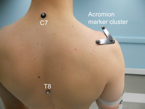
Figure 1: Position of the acromion marker cluster, C7 and T8 anatomical markers. This figure has been modified from Warner, M. B., Chappell, P. H. & Stokes, M. J. Measuring scapular kinematics during arm lowering using the acromion marker cluster. Hum. Mov. Sci. 31, 386-396, doi:http://dx.doi.org/10.1016/j.humov.2011.07.004 (2012).
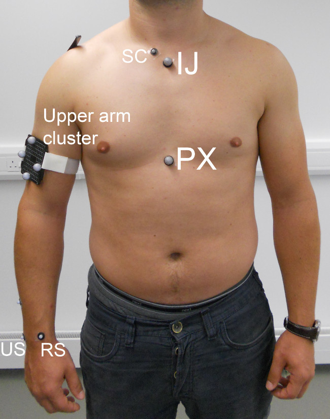
Figure 2: Marker locations for the sternal notch (IJ), xiphoid process (PX), sternoclavicular (SC), upper arm cluster, ulnar styloid (US), radial styloid (RS).
2. Participant Calibration
NOTE: Locations of the scapula’s anatomical landmarks need to be determined with respect to the acromion marker cluster. Calibration of the landmarks is required for each participant.
- Construct a calibration wand consisting of four reflective markers placed into a ‘T’ formation (Figure 3). Measure the distance from the tip of the calibration wand to the first wand marker.
- Palpate and locate the following anatomical landmarks as recommended by the International Society of Biomechanics33. Place the tip of the calibration wand on the landmark (Figure 3). Capture three seconds of data with the motion capture system ensuring the markers on the wand, the AMC and upper arm cluster are all visible to the cameras.
- Acromioclavicular joint (AC) — Place a hand on the clavicle, then move laterally until the point where the clavicle reaches the acromion. Place the tip of the wand at the joint between the clavicle and acromion.
- Acromion angle (AA) — Palpate along the spine of the scapula to the most lateral point. Place the tip of the wand on the dorsal aspect of the acromion at the most lateral point (Figure 3).
- Medial spine of the scapula (TS) — Palpate along the spine of the scapula to the most medial point. Place the tip of the wand at the point where the spine meets the medial border of the scapula.
- Inferior angle of the scapula (AI) — Palpate inferiorly along the medial border of the scapula. Place the tip of the wand on the most caudal point of the scapula.
- Medial epicondyle (EM) — With the participant’s elbow in 90° of flexion pointing forward, with their thumb pointing upwards, place a hand on the medial side of the elbow to locate the medial epicondyle. Place the tip of the wand on the most caudal point of the medial epicondyle.
- Lateral epicondyles (EL) — With the participant’s elbow in 90° of flexion pointing forward, with their thumb pointing upwards, place a hand on the lateral side of the elbow to locate the lateral epicondyle. Place the tip of the wand on the most caudal point of the lateral epicondyle.
- To determine the glenohumeral joint center, ask the participant to perform a circumduction movement with their upper arm with the elbow fully extended, from zero degrees arm elevation to approximately 40° arm elevation. They must perform this movement whilst aiming to minimize protraction/retraction and elevation/depression of the shoulder complex; the investigator can provide assistance if necessary. Record this movement for approximately 30 sec.
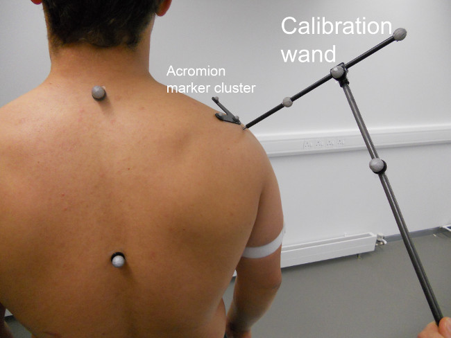
Figure 3: Calibration wand used to locate anatomical bony landmark with respect the acromion marker cluster (AMC).
3. Experiment Protocol
- Ask participant to perform arm elevation from zero to 120° arm elevation, and then lower their arm back down to rest by their side in the sagittal, frontal and scapular plane. The scapular plane is approximately 40° anterior to the frontal plane.
4. Post-processing of Kinematic Data
NOTE: The following steps detail the procedure needed to calculate scapular kinematics during the dynamic movement trials. These steps have been described and explored extensively within the literature21,33,34 and the purpose of the following section is to provide a synthesis and step-by-step guide to implementing the modeling steps required to obtain scapular kinematics. The application of these steps is conducted in relevant kinematic modeling software. The software contains commands to enable the creation of local coordinate systems, the conversion of coordinates from a global to local coordinate system, the conversion of coordinates from local to global coordinate systems and the calculation of Euler angle rotations. These steps will allow the scapula, humerus and thorax to be defined as rigid bodies. Subsequently rotation of the scapula with respect the thorax, and the humerus with respect thorax can then be determined.
- Using the coordinates of markers on the AMC, define an arbitrary local coordinate system for the AMC (Figure 4a). For each scapular anatomical landmark calibration trial, determine the location of the tip of the wand, which represents the location of the anatomical landmark, with respect the local coordinate system on the AMC using the following steps.
NOTE: Kinematic modeling software contain commands to enable the creation of local coordinate systems and conversion of coordinates from a global to a local coordinates, see Figure 4 for example commands.- Use the markers on the wand to create a local coordinate system for the wand (Figure 4a) using the following command in the kinematic modeling software: AMC= [AMCO,AMCA-AMCO,AMCO-AMCM,xyz] where AMCO, AMCA and AMCM are the labels given to the markers on the AMC.
- Using the kinematic modeling software, calculate the location of the tip of the wand in the global coordinate system. In the example provided this is 83 mm from the marker 1 (M1) along the X axis of the wand (Figure 4b); use the command: Wand = [M1,M1-M2,M3-M4,xyz] and Wandtip = M1+{83,0,0}*ATTITUDE(Wand) where M1, M2, M3 and M4 are the labels given to the markers on the wand.
- Determine the location of the tip of the wand with respect to the local coordinate system of the AMC ($%AA) (Figure 4c) using the modeling commands: $%AA = WandTip/AMC and PARAM($%AA).
- Repeat steps 4.1.1 to 4.1.3 for each scapular anatomical landmark.
- Determine the location of the medial and lateral epicondyles with respect to the humerus marker cluster, instead of the AMC, using the using the above steps.
- Use the dynamic calibration trial to calculate the location of the glenohumeral joint center with respect to the scapula. Calculate the position of the glenohumeral joint center, with respect to the scapula, as the pivot point of the helical axis between the humerus and scapula. For more details on this technique refer to Veeger35.
- Calculate the elbow joint center (ELJC) as the mid-distance between the lateral (EL) and medial epicondyles (EM) of the humerus; ELJC = (EM + EL) / 2.
- During the dynamic trials, use the known position of the anatomical landmarks with respect to the AMC to determine the location of the anatomical landmarks within the global coordinate system (Figure 5).
NOTE: Modeling software contain commands to enable conversion of coordinates from local coordinate systems to global coordinate systems, see Figure 5 for example commands.- Refer to Figure 5a that shows the location of the acromion angle landmark with respect to the AMC ($%AA) as described in point 4.1.
- Convert the location of $%AA virtual marker to the global coordinate system for each time point during the dynamic trial to create the acromion angle (AA) landmark (Figure 5b) using the following kinematic modeling command: AA = $%AA*AMC and OUTPUT(AA).
- Repeat steps 4.4.2 for each anatomical landmark.
- Define a local coordinate system for the thorax and scapula by calculating the unit vectors between the relevant markers to represent each axis for a given rigid body using the following kinematic modeling command: Scapula = [AA,TS-AA,AA-AI,zxy]. Thorax = [IJ,MUTHX-MLTHX,IJ-C7,yzx], where MUTHX is the mid-point between the IJ and C7 landmark and MLTHX is the mid-point between the PX and T8 landmarks.
NOTE: The axes definition are based on International Society of Biomechanics’ (ISB) recommendations33 (Table 1 and Figure 6).- Using a similar method, define a local coordinate system for the humerus using ‘Option 2’ as recommended by the ISB33.
NOTE: Option 2 requires a sufficient plane formed by the gleohumeral joint center, elbow joint center and the ulna styloid, i.e. a degree of elbow flexion is required. If the participant approaches full elbow extension, the humeral axes may become unstable and therefore ‘Option 1’ should be used (Table 1). See Wu et al. (2005) for further details.
- Using a similar method, define a local coordinate system for the humerus using ‘Option 2’ as recommended by the ISB33.
- Determine the orientation of the scapula relative to the thorax for each time point during the dynamic trial using the Euler angle decomposition method with a rotation sequence of internal rotation (Y), upward rotation (X’) and posterior tilt (Z’’)33 using the following kinematic modeling command: ScapularKin = - (Figure 7).
- Determine the orientation of the humerus with respect to the thorax during the dynamic trial using a non-cardan rotation sequence of Y (plane of elevation), X’ (elevation) and Y’’ (axial rotation)36 using relevant kinematic modeling software.
NOTE: A macro is available to download from the manufacturer in order to determine non-cardan rotation sequences within the kinematic modeling software used in this manuscript.
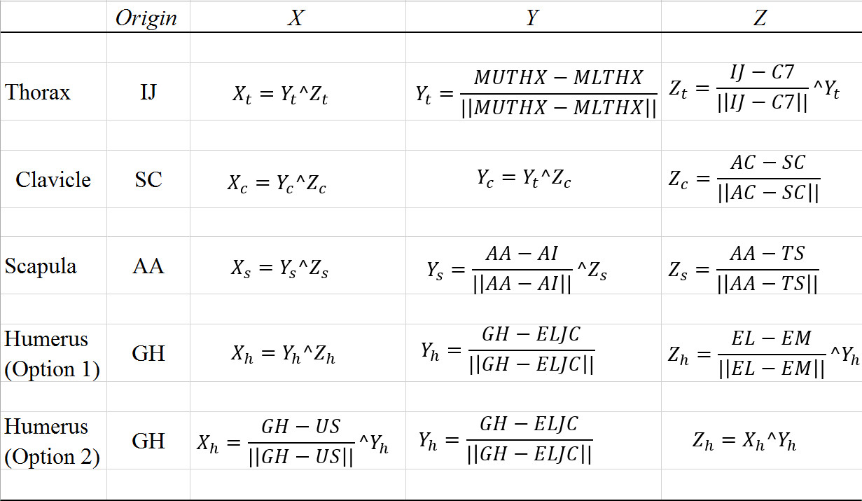
MUTHX = mid-point between IJ and C7. MLTHX = mid-point between PX and T8. GH = glenohumeral joint center. ELJC = elbow joint center.
Mathematical operators:
^ = cross product of two vectors
|| = absolute value of a vector
Table 1: Local coordinate system for each rigid segment.
5. Data Reduction and Analysis
NOTE: The following data reduction and analysis steps are performed in numerical modeling software (such as MATLAB) that allows manipulation of data matrices. The kinematic data is divided into the elevation and lowering phases of humeral movement, time normalized for each phase of movement, then scapular kinematics are expressed relative to humeral elevation angle.
- Determine the elevation and lowering phase of the humeral elevation as described below (Figure 8). These phases are determined from the angular velocity of the humeral elevation angle (Figure 8). See ElevationLoweringPhases.m function file.
- Determine the start of humeral elevation when the angular velocity of the humerus exceeds a threshold 2% of the maximal humeral angular velocity.
- Determine the end of the elevation phase as the point at which the humeral angular velocity falls below 2% of the maximal humeral angular velocity, or when humeral elevation exceeds 120°.
- Determine the start of the humeral lowering phase when the angular velocity falls below 2% of the minimum angular velocity, or the point at which humeral elevation falls below 120°.
- Determine the end of the lowering phase when the angular velocity exceeds 2% of the minimum angular velocity.
- Normalize the data by interpolating the kinematic data in each phase of movement to 101 data points (Figure 9). See Time_normalisation.m function file.
- Express scapular kinematics in relation to humeral elevation by plotting the arm angle (degrees) vs. upward rotation (degrees) (Figure 10). See PlotScapHumRhythm.m function file.
Access restricted. Please log in or start a trial to view this content.
Results
Fifteen participants who had no known history of shoulder, neck or arm injuries were recruited onto the study (Table 2). To assess intra-rater (between-day) reliability, participants attended two data collection sessions separated by at least 24 hours and a maximum of 7 days. During each data collection session, the same investigator performed the protocol for attaching reflective markers, the acromion marker cluster and anatomical landmark calibrations, as detailed above. The reliability of the kinemati...
Access restricted. Please log in or start a trial to view this content.
Discussion
The choice of methodology for determining scapular kinematics is crucial, and consideration of the validity, reliability and its appropriateness for the research study should be given. Various methods have been adopted throughout the literature but each method has its limitations. The acromion marker cluster overcomes a number of these limitations, such as projection errors from 2D imaging or requiring repeated interpretation of the location of the scapula by providing non-invasive dynamic kinematic measurement of the sc...
Access restricted. Please log in or start a trial to view this content.
Disclosures
None of the authors had any affiliation with any organization that could influence the outcome of this work.
Acknowledgements
This work lies within the multidisciplinary Southampton Musculoskeletal Research Unit (Southampton University Hospitals Trust/University of Southampton) and the Arthritis Research UK Centre for Sport, Exercise and Osteoarthritis. The authors wish to thank their funding sources; Arthritis Research UK for funding of laboratory equipment (Grant No: 18512) and Vicon Motion System, Oxford UK for providing funding for a PhD studentship (M.Warner). The authors also wish to thank the participants, and Kate Scott and Lindsay Pringle for their help with participant recruitment.
Access restricted. Please log in or start a trial to view this content.
Materials
| Name | Company | Catalog Number | Comments |
|---|---|---|---|
| Passive marker capture system | Vicon Motion Systems | N/A | |
| Nexus | Vicon Motion Systems | N/A | Data capture software |
| Bodybuilder | Vicon Motion Systems | N/A | Modeling software |
| 14 mm retro reflective markers | Vicon Motion Systems | VACC-V162B | |
| 6.5 mm retro reflective markers | Vicon Motion Systems | VACC-V166 | |
| Calibration wand | Vicon Motion Systems | N/A | |
| Plastic base | N/A | N/A | Constructed 'in-house' |
| Matlab | Mathworks | N/A | Numerical modelling software |
References
- Kibler, W. B., et al. Clinical implications of scapular dyskinesis in shoulder injury: the 2013 consensus statement from the 'scapular summit'. British Journal of Sports Medicine. 47, 877-885 (2013).
- Luckasiewicz, A. C., McClure, P. W., Michener, L. A., Pratt, N., Sennett, B. Comparison of 3-dimensional scapular position and orientation between subjects with and without shoulder impingement. Journal of Orthopaedic & Sports Physical Therapy. 29, 574-586 (1999).
- Ludewig, P. M., Cook, T. M. Alterations in shoulder kinematics and associated muscle activity in people with symptoms of shoulder impingement. Physical Therapy. 80, 276-291 (2000).
- McClure, P. W., Bialker, J., Neff, N., Williams, G., Karduna, A. R. Shoulder function and 3-dimensional kinematics in people with shoulder impingement syndrome before and after a 6-week exercise program. Physical Therapy. 84, 832-848 (2004).
- Lin, J. J., et al. Functional activity characteristics of individuals with shoulder dysfunctions. Journal of Electromyography and Kinesiology. 15, 576-586 (2005).
- Tate, A. R., McClure, P. W., Kareha, S., Irwin, D., Barbe, M. F. A clinical method for identifying scapular dykinesis, Part 2: Validity. Journal of Athletic Training. 44, 165-173 (2009).
- Timmons, M. K., et al. Scapular kinematics and subacromial-impingement syndrome: a meta-analysis. Journal of Sports Rehabilitation. 21, 354-370 (2012).
- Endo, K. Y. K., Yasui, N. Influence of age on scapulo-thoracic orientation. Clinical Biomechanics. 16, 1009-1013 (2004).
- Lovern, B., Stroud, L. A., Evans, R. O., Evans, S. L., Holt, C. A. Dynamic tracking of the scapula using skin-mounted markers. Proceedings of the Institute of Mechanical Engineers. 223, 823-831 (2009).
- Inman, V. T., Sanders, J. B., Abbott, L. C. Observations on the function of the shoulder joint. Journal of Bone and Joint Surgery (Am). 26, 1-30 (1944).
- Saha, A. K. Mechanics of elevation of the glenohumeral joint. Acta Orthopaedica Scandanavia. 44, 668(1973).
- Freedman, L., Munro, R. R. Abduction of the arm in the scapular plane: scapular and glenohumeral movements. A roentgenographic study. Journal of Bone and Joint Surgery (Am). 48, 1503-1510 (1966).
- Poppen, N. K., Walker, P. S. Normal and abnormal motion of the shoulder. Journal of Bone and Joint Surgery (Am). 58, 195-201 (1976).
- Graichen, H., et al. Magnetic resonance-based motion analysis of the shoulder during elevation). Clinical Orthopedic Related Research. 370, 154-163 (2000).
- Youdas, J. W., Carey, J. R., Garrett, T. R., Suman, V. J. Reliability of goniometric measurements of active arm elevation in the scapula plane obtained in a clinical setting. Arch. Phys. Med. Rehabil. 75, 1137-1144 (1994).
- Doody, S. G., Freedman, L., Waterland, J. C. Shoudler movement during abduction in the scapula plane. Arch. Phys. Med. Rehabil. 51, 595-604 (1970).
- Karduna, A. R., McClure, P. W., Michener, L. A., Sennett, B. Dynamic measurements of three-dimensional scapular kinematics: a validation study. Journal of Biomechanical Engineering. 123, 184-191 (2001).
- McClure, P. W., Michener, L. A., Sennett, B., Karduna, A. R. Direct 3-dimensional measurement of scapular kinematics during dynamic movements in vivo. Journal of Shoulder and Elbow Surgery. 10, 269-277 (2001).
- Bourne, D. A., Choo, A. M. T., Regan, W. D., MacIntyre, D. L., Oxland, T. R. Three-dimensional rotation of the scapula during functional movements: an in vivo study in healthy volunteers. Journal of Shoulder and Elbow Surgery. 16, 150-162 (2007).
- Braman, J. P., Engel, S. C., LaPrade, R. F., Ludewig, P. M. In vivo assessment of scapulohumeral rhythm during unconstrained overhead reaching in asymptomatic subjects. Journal of Shoulder and Elbow Surgery. 16, 960-967 (2009).
- Ludewig, P. M., Hassett, D. R., LaPrade, R. F., Camargo, J. A., Braman, J. P. Comparison of scapular local coordinate systems. Clinical Biomechanics. 25, 415-421 (2010).
- Ludewig, P. M., et al. Motion of the shoulder complex during multiplanar humeral elevation. The Journal of Bone and Joint Surgery. 91, 378-389 (2009).
- Johnson, G. R., Stuart, P. R., Mitchell, S. A method for the measurement of three-dimensional scapular movement. Clinical Biomechanics. 8, 269-274 (1993).
- Helm, F. C., Pronk, G. M. Three-dimensional recording and description of motions of the shoulder mechanism. Journal of Biomechanical Engineering. 117, 27-40 (1995).
- McQuade, K. J., Smidt, G. L. Dynamic Scapulohumeral rhythm: The effects of external resistance during elevation of the arm in the scapular plane. Journal of Orthopaedic & Sports Physical Therapy. 27, 9(1998).
- Matsui, K., Shimada, K., Andrew, P. D. Deviation of skin marker from bone target during movement of the scapula. Journal of Orthopaedic Science. 11, 180-184 (2006).
- Meskers, C. G. M., Jvan de Sande, M. A., de Groot, J. H. Comparison between tripod and skin-fixed recording of scapular motion. J. Biomech. 40, 941-948 (2007).
- Andel, C. J., van Hutten, K., Eversdijk, M., Veeger, D. J., Harlaar, J. Recording scapular motion using an acromion marker cluster. Gait and Posture. 29, 123-128 (2009).
- Warner, M. B., Chappell, P. H., Stokes, M. J. Measuring scapular kinematics during arm lowering using the acromion marker cluster. Hum. Mov. Sci. 31, 386-396 (2012).
- Worsley, P., et al. Motor control retraining exercises for shoulder impingement: effects on function, muscle activation, and biomechanics in young adults. Journal of Shoulder and Elbow Surgery. 22, e11-e19 (2013).
- Shaheen, A. F., Alexander, C. M., Bull, A. M. J. Effects of attachment position and shoulder orientation during calibration on the accuracy of the acromial tracker. J. Biomech. 44, 1410-1413 (2011).
- Prinold, J. A. I., Shaheen, A. F., Bull, A. M. J. Skin-fixed scapula trackers: A comparison of two dynamic methods across a range of calibration positions. J. Biomech. 44, 2004-2007 (2011).
- Wu, G., et al. ISB recommendation on definitions of joint coordinate systems of the various joints for the reporting of human joint motion - Part II: shoulder, elbow, wrist and hand. J. Biomech. 38, 981-992 (2005).
- Karduna, A. R., McClure, P. W., Michener, L. A. Scapular kinematics: effects of altering the Euler angle sequence of rotations. J. Biomech. 33, 1063-1068 (2000).
- Veeger, H. E. J. The position of the rotation center of the glenohumeral joint. J. Biomech. 33, 1711-1715 (2000).
- Doorenbosch, C. A. M., Harlaar, J., Veeger, H. E. J. The globe system: an unambiguous description of shoulder positions in daily life movements. J. Rehabil. Res. Dev. 40, 147-156 (2003).
- Kadaba, M. P., et al. Repeatability of kinematic, kinetic, and electromyographic data in normal adult gait. Journal of Orthopaedic Research. 7, 849-860 (1989).
- Schwartz, M. H., Trost, J. P., Wervey, R. A. Measurement and management of errors in quantitative gait data. Gait and Posture. 20, 196-203 (2004).
- Jaspers, E., et al. The reliability of upper limb kinematics in children with hemiplegic cerebral palsy. Gait and Posture. 33, 568-575 (2011).
- Thigpen, C. A., Gross, M. T., Karas, S. G., Garrett, W. E., Yu, B. The repeatability of scapular rotations across three planes of humeral elevation. Research in Sports Medicine. 13, 181-198 (2005).
- Groot, J. H. The variability of shoulder motions recorded by means of palpation. Clinical Biomechanics. 12, 461-472 (1997).
Access restricted. Please log in or start a trial to view this content.
Reprints and Permissions
