Quantification of Heavy Metals and Other Inorganic Contaminants on the Productivity of Microalgae

Summary

Integration of microalgal cultivation with industrial flue gas will ultimately introduce heavy metals and other inorganic compounds into the growth media. This study presents a procedure used to determine the end fate and impact of heavy metals and inorganic contaminants on the growth of Nannochloropsis salina grown in photobioreactors.

Abstract

Increasing demand for renewable fuels has researchers investigating the feasibility of alternative feedstocks, such as microalgae. Inherent advantages include high potential yield, use of non-arable land and integration with waste streams. The nutrient requirements of a large-scale microalgae production system will require the coupling of cultivation systems with industrial waste resources, such as carbon dioxide from flue gas and nutrients from wastewater. Inorganic contaminants present in these wastes can potentially lead to bioaccumulation in microalgal biomass negatively impact productivity and limiting end use. This study focuses on the experimental evaluation of the impact and the fate of 14 inorganic contaminants (As, Cd, Co, Cr, Cu, Hg, Mn, Ni, Pb, Sb, Se, Sn, V and Zn) on Nannochloropsis salina growth. Microalgae were cultivated in photobioreactors illuminated at 984 µmol m^-2 sec^-1 and maintained at pH 7 in a growth media polluted with inorganic contaminants at levels expected based on the composition found in commercial coal flue gas systems. Contaminants present in the biomass and the medium at the end of a 7 day growth period were analytically quantified through cold vapor atomic absorption spectrometry for Hg and through inductively coupled plasma mass spectrometry for As, Cd, Co, Cr, Cu, Mn, Ni, Pb, Sb, Se, Sn, V and Zn. Results show N. salina is a sensitive strain to the multi-metal environment with a statistical decrease in biomass yieldwith the introduction of these contaminants. The techniques presented here are adequate for quantifying algal growth and determining the fate of inorganic contaminants.

Introduction

Compared to traditional terrestrial crops microalgae have been shown to achieve higher biomass and lipid yields due to inherent higher solar conversion efficiencies^1,2. Cultivation of microalgae at high productivity rates requires the supply of various nutrients including an external carbon source. It is expected that large-scale growth facilities will be integrated with industrial waste streams such as industrial flue gas in order to minimize production costs and at the same time provide environmental remediation. Industrial waste carbon is typically in the form of gaseous carbon dioxide and can contain contaminants that have the potential to negatively impact microalgae production. Specifically, flue gas derived from coal will have a variety of contaminants including but not limited to combustion products water and carbon dioxide, as well as oxides of sulphur and nitrogen, fine dust, organic contaminants such as dioxins and furans, and inorganic contaminants such as heavy metals. The impact of the majority of these contaminants including inorganics with some of them known as heavy metals on microalgae productivity have not been explored. Some of these elements can be nutrients at appropriate concentrations, however at higher concentrations they can produce cell dysfunction and even death³.

The integration of microalgae with industrial flue gas has the potential to directly introduce inorganic contaminants into growth media. Coal based flue gas has a variety of inorganic elements (e.g., As, Cd, Co, Cr, Cu, Hg, Mn, Ni, Pb, Sb, Se, Sn, V and Zn) at various concentrations some of which, in low concentration, represent nutrients for microalgae growth. Inorganic contaminants have a high affinity to bind to microalgae and further be sorbed internally through nutrient transporters. Some inorganic contaminants (i.e., Co, Cu, Zn and Mn) are nutrients that form part of enzymes involved in photosynthesis, respiration and other functions^3,4. However, in excess metals and metalloids can be toxic. Other elements, such as Pb, Cd, Sn, Sb, Se, As and Hg, are not known to support cell function in any concentration and represent non-nutrient metals which could negatively impact culture growth^3,5,6. The presence of any of these contaminants has the potential to produce negative effects on microalgae cell function. Furthermore, the interaction of multiple metals with microalgae complicates growth dynamics and has the potential to impact growth.

Large-scale economics have been directly linked to the productivity of the cultivation system^7-19. Moreover, medium recycle in the microalgae growth system for either open raceway ponds (ORP) or photobioreactors (PBR) is critical as it represents 99.9 and 99.4% of the mass, respectively²⁰. The presence of inorganic contaminants in the media could ultimately limit microalgae productivity and the recycling of media due to contaminant build up. This study experimentally determined the impact of 14 inorganic contaminants (As, Cd, Co, Cr, Cu, Hg, Mn, Ni, Pb, Sb, Se, Sn, V and Zn), at concentrations expected from the integration of microalgae cultivation systems with coal derived flue gas, on the productivity of N. salina grown in airlift PBRs. The contaminants used in this study have been shown to not only be present in coal-based flue gas but municipal waste-based flue gas, biosolids-based flue gas, municipal wastewater, produced water, impaired groundwater and seawater^21-23. The concentrations used in this study are based on what would be expected if microalgae growth systems were integrated with a coal based CO₂ source with an uptake efficiency demonstrated in commercial PBR systems²⁰. Detailed calculations supporting the concentrations of the heavy metals and inorganic contaminants are presented in Napan et al.²⁴ Analytical techniques were used to understand the distribution of the majority of the metals in the biomass, media and environment. The methods presented enabled the assessment of productivity potential of microalgae under inorganic contaminant stress and quantification of their end fate.

Protocol

1. Growth system

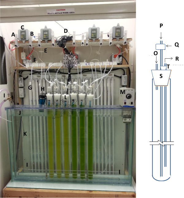
Figure 1. Microalgae growth system. (A) air rotometer, (B) CO₂ rotometer, (C) pH controller with solenoid, (D) data logger, (E) in-line air filters, (F) air distribution header, (G) fluorescent light bank, (H) pH meters, (I) cooling system, (J) water bath, (K) thermocouple wire, (L) air lift photobioreactor, (M) heater, (N) walk-in fume hood, (O) vent, (P) air delivery capillary tube, (Q) air filters, (R) sampling tube, (S) PBR silicone lid, and (T) pH well in silicone lid. Please click here to view a larger version of this figure.

1. Build the following microalgae experimental growth system (Figure 1).
   1. Acquire twelve airlift PBRs consisting of glass tube reactors 4.5 cm in diameter and 80 cm in height with a cultivation capacity of 1.1 L with silicone lids. Acquire pre-cut glass capillary tubes (5 mm external diameter and 1 mm internal diameter) of 10 cm (3 per PBR) and 85 cm (1 per PBR) in length.
   2. Freeze silicone lids in a -80 °C freezer. Lubricate a drill bit with glycerol and while lids are frozen drill 3 holes to host the vent, sampling and gas delivery capillary tubes, and 1 hole of 17 mm diameter to host a pH probe.
   3. Insert the 3 capillary tubes in place with the longest tube extending 2 cm from the bottom of the PBR. In the other capillary tube add a silicon tube with a capillary tube attached to the other end extending to a desired sampling point. Cover the hole for the pH meter with a silicone stopper size 21D.
   4. Humidify ambient air by bubbling it through water and deliver the humidified air to the air distribution header. Pass the gas through a 0.2 µm filter and deliver it to the algal suspension through the longest glass delivery capillary tube.
   5. Deliver compressed CO₂ into the humidified air stream in order to maintain a neutral pH of 7.0 ± 0.1 in the culture suspension. Control the rate of CO₂ delivery with an automated CO₂ dispensary system (pH controller) that opens a magnetic solenoid when the algal culture reaches pH 7.1 and closes at pH 6.9.
   6. Provide light using 24 T5 fluorescent lamps that result in an average illumination of 984 µmol m^-2 sec^-1 similar to peak outdoor conditions.
   7. Immerse the PBRs in a water bath in order to maintain a constant temperature of approximately 25 °C. Control the temperature of the system by using a recirculating chiller and an automated heating recirculating water bath unit control.
   8. Monitor temperature and pH in real-time and record with a data logger.
   9. Ensure that all components of the microalgae growth system are properly working, especially before harvesting microalgae inoculum or preparing inorganic contaminants as they cannot be preserved.

2. Lab Ware Preparation

1. Wash volumetric flasks, PBRs, carboys and any containers, with soap and tap water. Rinse with deionized water (DW).
2. Acid rinse the lab ware in order to eliminate any traces of inorganic contaminants. This can be done by one of two ways:
   1. Soak lab ware O/N in 10% trace metal grade nitric acid (CAUTION: Do not breath fumes, concentrated nitric acid can produce severe burning and toxic fumes, work in a fume hood using nitrile gloves, goggles and lab coat).
   2. Soak lab ware for 15 min in 50% trace metal grade nitric acid.
   3. Rinse the lab ware with DW thoroughly at least 3 times making sure all acid is removed. It is critical that PBRs are thoroughly rinsed, especially the sampling tubes and the capillary tubes. Failure to do this will produce acidification of the medium and possible inhibition of growth. Test the pH of the rinse water to verify all acid has been removed.
   4. Sterilize PBRs, containers and flasks by autoclaving them at 120 °C and standard atmospheric pressure for at least 30 min.

3. N. salina Medium Preparation

1. Preparation of solution A: Partially fill a 1 L volumetric flask with DW. Insert a magnetic stir bar and add the chemicals shown in Table 1 one after the other. Ensure that each ingredient dissolves before the addition of the next constituent. Remove the magnet and fill the flask to the 1 L volume mark.

Component	Amount to add (g)	Final concentration (g/L)
H3BO3	0.900	0.900
Na2MoO4·2H2O	0.012	0.012
MnCl2·4H2O	0.300	0.300
ZnSO4·7H2O	0.060	0.060
CuSO4·5H2O	0.020	0.020

Table 1: Solution A recipe. Quantities are amounts needed in the preparation of 1 L of concentrated solution. 

2. Preparation of vitamin solution: In three separate volumetric flasks add the vitamins as shown in Table 2. Filter each vitamin solution through a sterile 0.2 µm syringe filter to a sterile container. Preserve vitamins at -4 °C in the dark.

Vitamins	Amount (mg)	Final volume (mL)	Final vitamin concentration (mg/L)
Biotin	12.22	500	24.43
Vitamin B12	13.50	100	135.00
Thiamine hydrochloride	977.63	500	1,955.27

Table 2: Vitamin solution recipe. Quantities are amounts needed for the preparation of concentrated solution. 

3. Partially fill a 20 L autoclavable container with DW and insert a magnetic stir bar. Place the container on top of a magnetic stirrer plate and add the chemicals shown in Table 3 (except the vitamins), adding them one after the other and after each fully dissolves. Fill the container to reach 20 L.

Component	Amount to add to medium	Unit
NaCl	350.00	g
CaCl2·2H2O	3.00	g
KCl	9.60	g
Na2SiO3·9H2O	1.14	g
MgSO4·7H2O	29.60	g
KNO3	20.40	g
KH2PO4	1.36	g
Ammonium ferric citrate	0.10	g
Solution A	20.00	ml
Biotin solution*	818.00	µl
Vitamin B12 solution*	296.20	µl
Thiamine hydrochloride solution*	521.60	µl
* Add to cooled autoclaved media

Table 3: N. salina medium recipe. Quantities are amounts needed in the preparation of 20 L of nutrient-rich medium. 

4. Sterilize the medium by autoclaving for 30 min at 120 °C and atmospheric pressure. Let the medium cool down to RT.
5. Place the container on a magnetic stirrer plate. Add the vitamins prepared in step 3.2 and let the medium mix thoroughly.

4. Inorganic contaminants stock preparation

1. Partially fill the volumetric flasks indicated in Table 4 with DW and add the individual salt listed. Fill with DW to the required final volume and mix thoroughly. Do not preserve these stocks as some elements adsorb to flask walls
   CAUTION: Several inorganic contaminants used in this protocol are carcinogenic, teratogenic and mutagenic, wear a face mask, gloves and lab coat when handling salts.

Analyte	Salt source	Volume of stock to prepare           (L)	Salt to add to the flask                     (mg salt)	Analyte concentration added to the culture               (mg analyte/L)
As	NaAsO2	0.1	14.8	7.74E-02
Cd	CdCl2	0.5	13.5	1.50E-02
Co	CoCl2.6H2O	0.5	34.7	1.56E-02
Cr	Na2Cr2O7·2H2O	0.1	40.6	1.29E-01
Cu	CuCl2.2H2O	0.1	38.3	1.30E-01
Hg	HgCl2	1.0	14.6	9.80E-03
Mn	MnCl2.4H2O	0.1	58.8	1.49E-01
Ni	NiCl2.6H2O	0.1	112.0	2.51E-01
Pb	PbCl2	0.5	39.9	5.41E-02
Sb	Sb2O3	0.5	26.7	4.06E-02
Se	Na2SeO3	0.5	11.8	9.80E-03
Sn	SnCl2.2H2O	0.5	3.9	3.76E-03
V	V2O5	0.1	22.2	1.13E-01
Zn	ZnCl2	0.1	99.9	4.36E-01

Table 4: Concentrated inorganic contaminants stock preparation. Addition of 1 ml of this concentrated stock to the 1.1 L PBR medium produces the final concentration shown in the last column. 

2. Sterilize the inorganic contaminant stocks by passing the solution through a sterile 0.2 µm syringe filter and collect the filtrate in a sterile tube.

5. N. salina Inoculum Production

1. In a 500 ml Erlenmeyer flask add 200 ml of medium prepared in step 3 and then add 3 g of agar. Cover the flask with aluminum foil and autoclave for 20 min at 120 °C. Pour the solution into sterile petri-dishes and let it cool until it solidifies. This should be completed be a sterile hood or at least near a flame in a clean environment to reduce risk of contamination.
2. Streak N. salina cells in sterile petri-dishes prepared in step 5.1 using a sterile seeding loop. Place the petri-dish cultures on a table illuminated with T12 lights maintained at RT. Let microalgae grow until colonies are visible.
3. Transfer colonies to sterile baffled Erlenmeyer flasks containing 200 ml of nutrient rich medium prepared in step 3 and keep them on an illuminated shaker table (1,000 RPM). Let the culture grow until medium becomes green.
4. Transfer the microalgae to a 1.1 L sterile PBR. Place the PBR in an inoculum water bath illuminated at 200 µmol m^-2 sec^-1 with T8 fluorescent lights and maintained at 23 °C by a recirculating chiller and an automated heating recirculating water bath control. Adjust the air and CO₂ rotometers to 2.5 L min^-1 and 25 cc min^-1, respectively.
5. After a week of growth split biomass into new 1 .1 L PBRs containing new medium and let it grow until a total of at least 28 g of dry weight biomass are obtained between the two reactors which can be determined through optical density.
6. Harvest the inoculum biomass by centrifugation at 2,054 × g for 15 min at 10 °C using sterile centrifuge bottles and sterile techniques to avoid contamination. Dispose of the supernatant and continue cell concentration as needed.
7. Once all biomass is centrifuged, re-suspend the cells in 300 ml of fresh sterile medium.
8. Dilute 0.1 ml of microalgal culture in 3 ml of DW and then dilute 0.1 ml of this new solution in 3 ml of DW. Ensure the sample is thoroughly mixed. Measure the optical density (OD) of the microalgae concentrate at 750 nm () immediately using a spectrophotometer.
9. Use equation (1) to determine the amount of biomass in the concentrate.
   Note: Equation (1) was obtained from the linear regression between versus total suspended solids ( in g/L^-1) for N. Salina (R²=0.9995). Equation 1 was developed for the spectrophotometer model in the Materials Table, generate a new calibration if using another spectrophotometer model.
   1. Using equation (2) calculate the volume of microalgae concentrate (in L) needed to obtain a 4 g/L^-1 culture density in a PBR of 1.1 L volume (in L).

10. Using sterile techniques, add the volume of microalgae concentrate found in the step 5.9 to an autoclaved PBR to reach an initial culture density of 4 g/L^-1. Fill PBR with medium to 1.1 L. Repeat this step until 6 PBRs are inoculated. Place the PBRs in the inoculum water bath.
11. Let the microalgae in the PBRs grow for 8 days and then harvest the biomass (by repeating steps 5.6 to 5.7). Repeat step 5.8 to calculate the initial inoculum volume for an initial culture density of 1 g/L^-1.

6. Experimental Reactors

1. Using sterile techniques add approximately 1 L of medium prepared in step 3 to each of the 12 acid-rinsed sterile PBRs. Place the PBRs in the water bath of the experimental growth system. Turn sparge air on at 1.5 L min^-1.
2. Sterilize a calibrated pH meter by cleaning it with 70% ethanol. Measure the pH of the medium in the PBR and ensure pH is approximately 7.0; if not, repeat step 2 to remove acid leached from the acid rinsing step.
3. Calibrate each pH controller using buffer pH 7, disinfect the probes using ethanol (70%) and then insert them in the PBRs lids.
4. To each PBR (except the control PBRs) add 1 ml of each of the sterile inorganic contaminants stocks prepared in step 4. Let the contaminants thoroughly mix in the PBR. The final concentration of the inorganic contaminants in the PBRs are shown in the last column in Table 4, and are the estimated maximum concentrations expected from a coal-fired power plant integration.
5. Add 14 ml of sterile DW to the control PBRs.
6. Add the concentrated microalgae inoculum obtained in step 5.11 to the experimental PBRs in order to obtain an initial culture density of 1 g/L^-1. Let biomass mix thoroughly.
7. Turn high light intensity lights (of 984 µmol m^-2 sec^-1) and pH controllers on and adjust CO₂ to 30 cc min¹. Increase the CO₂ flow to 50 cc min^-1 from day 3 afterwards. Initial low CO₂ flow rate is critical in order to avoid large changes in pH due to delays in gas/liquid transfer and pH measurement.
8. Measure and take samples as needed. Make sure to mark the water level after sampling. (CAUTION: some inorganic contaminants in the PBR are carcinogenic, teratogenic and mutagenic; use gloves and capped containers when handling samples).
9. Add sterile DW daily to the PBRs in order to compensate for losses due to evaporation.
10. After 7 days of growth, harvest the biomass by centrifugation at 9,936 × g and preserve both, biomass and supernatant medium, at -80 °C.
11. Freeze dry the biomass at 0.1 mbar and -50 °C O/N. Powder the biomass (use a spatula to powder biomass inside the centrifuge tube). Preserve freeze dried biomass at -80 °C.

7. Microwave Assisted Digestion of Samples

The digestion of the biomass samples is required as a pre-processing step for ICP-MS analysis.
Note: These steps use a closed vessel microwave digestion system with controlled pressure relief. (CAUTION: High pressures develop during acid digestion, inspect the physical integrity of the digestion vessels and shields, and reshape the microwave digestion vessel lids before every use).

1. Wash Teflon microwave digestion vessels with soap and water, rinse with DW and let vessels air dry. To remove trace metal contamination in the vessels digest acid as described in the following steps.
2. Reshape the microwave digestion vessel lids and close the vials tightly.
3. Add 10 ml of nitric acid to each.
4. Introduce the vessel in the safety shield. Ensure that no biomass, water or any reagents are left on the walls of the safety shield or in the outer walls of the digestion vessels in order to avoid damage to the safety shield. Cap the safety shield with the safety valve making sure the spring in the vial is flush. Locate the shield on the rotor with the cap vents pointing outward in the outer row and inwards in the inner row.
5. On vessel number one, insert the ceramic thermowell and the temperature sensor. This thermometer monitors the actual internal temperature in the vial and serves as the controlling parameter to execute the digestion program. Ensure that vial number one contains the same sample and reagent amounts as the other vials.
6. Input the digestion parameters shown in Table 5 and start digestion. When the program has finished, air cool the vials until they reach RT.

Step	Vials rinsing			Sample digestion
	Temperature (°C)	Time (min)	Max. power (W)	Temperature (°C)	Time (min)	Max. power (W)
1	RT to 190	25	1,000	RT to 180	15	1,000
2	190	10	1,000	180	15	1,000
Exhaust	-	20	-	-	20	-

Table 5: Parameters used in the microwave digestion program.

7. Inside a fume hood, insert the pressure relief tool on the shield cap with the cap vents point away from you. Once pressure is released open the cap (CAUTION: Always open digested vials inside fume hood since biomass digestion using acid produces toxic fumes).
8. Dispose of the acid. Rinse the Teflon vessels with DW 3 times. Let vials air dry.
9. To digest biomass, add 50 mg of freeze dried biomass to microwave digestion vessels. For quality control (QC) prepare the following vials: in two different vials add either 5 ml of Level 7 ICPMS or 5 ml of Level 7 Hg CVAAS standard prepared in steps 9.1 and 10.1 (the digested solution from this vial is called the laboratory fortified blank (LFB)), leave another vial empty (the digested solution from this vial is called the laboratory reagent blank (LRB)).
10. To digest medium, add 10 ml supernatant medium to dry acid rinsed microwave digestion vessels. For quality control (QC) prepare the following vials: In two different vials add 5 ml of Level 7 ICPMS or CVAAS metal standard prepared in step 9.1 and 10.1 (the digested solution from this vial is called the LFB), to another vial add 10 ml of DW (the digested solution from this vial is called the LRB).
11. Reshape the microwave digestion vessel lids and close the vials tightly.
12. Add 7 ml of concentrated trace metal grade nitric acid and 3 ml hydrogen peroxide to each vial. Homogenize the contents by gently swirling the solution. Digest the contents of the vials by repeating steps 7.4 to 7.7 (use the microwave digestion parameters for sample digestion in Table 5).
13. Add digested sample to a 25 ml volumetric flask, rinsing the vessels with DW for increased recovery. Fill the volumetric flask with DW to the mark.
14. Transfer digested samples to a capped container. Preserve samples at 4 °C until analysis can be completed. For this study analysis is done the same day for Hg and within three days for the other elements.

8. Quality Control (QC) Samples

Note: Analyze QC samples in order to assure reliability of the results from experimental samples.

1. Partially fill an acid rinsed 1 L volumetric flask with DW. Add 280 ml of concentrated trace metal grade nitric acid and mix thoroughly (this solution is also called the blank solution) (CAUTION: always add acid to water, never add water to acid as the exothermic reaction can be violent). Let solution cool to RT.
2. In addition to QC samples prepared in steps 7.9 and 7.10, prepare the following QC samples.
   1. For the continuing calibration verification (CCV): Fill a polystyrene tube with calibration standard (for preparation see step 9.2 and 10.1). Put the Hg standard solution on the CVAAS rack and the ICPMS standard solution in the ICPMS autosampler.
   2. For the continuing calibration blank (CCB): Fill two polystyrene tubes (16 ml) with the blank (solution prepared in step 8.1). Place one sample in the CVAAS rack and the other sample in the ICPMS autosampler.
   3. For the laboratory-fortified matrix (LFM): Randomly choose 1 sample of every 12 samples for each type of sample (i.e., biomass or medium) and use it to prepare a LFM. For ICPMS, add 0.5 ml of ICPMS standard Level 7 and 3 ml of digested experimental sample (from either biomass or medium) to a polystyrene tube.
   4. Mix contents and place the vials on the ICPMS autosampler. For CVAAS, add 2 ml Hg standard Level 7 and 6 ml of digested experimental sample (from either biomass or medium) to a polystyrene tube. Mix contents and place vials on the CVAAS rack.
   5. For the duplicate samples: Randomly choose 1 sample of every 12 samples for each type of matrix (e.g., biomass, medium, LFM or any diluted matrix) and duplicate the vial. Place the repeated vials in the ICPMS autosampler or the CVAAS rack.
   6. For the duplicate samples: Randomly choose 1 sample of every 12 samples for each type of matrix (e.g., biomass, medium, LFM or any diluted matrix) and duplicate the vial. Place the repeated vials in the ICPMS autosampler or the CVAAS rack.
3. Define the data quality criteria for the study. For the present study duplicate the quality criteria established by Eaton, Clesceri, Rice and Greenberg ²⁵. The parameters established for the QC are: percent difference (%D) for CCV within ± 10%²⁵ (with exception of Pb and Sb, see discussion), LFB percent recovery (%R) within ± 70-130%²⁵, LFM percent recovery (%R) within 75-125%²⁵, and relative percent difference (RPD) within ± 20%²⁵, and a continuing calibration blank (CCB) below method reporting limit (MRL)²⁵. See calculation equations in step 9.7.

9. Quantification by Inductively Coupled Plasma Mass Spectrometry (ICPMS)

1. On the day of analysis, transfer approximately 5 ml of digested sample to polystyrene tubes and place them in the ICPMS autosampler. Add approximately 15 ml of digested samples to polystyrene tubes and place them in the CVAAS rack.
2. The same day of analysis prepare the calibration standards. Add purchased ICPMS standard solution and refill with blank (solution prepared in step 8.1) as described in Table 6 (see standard solution description in Material Table) to acid-rinsed volumetric flasks.

Parameter	Level 1	Level 2	Level 3	Level 4	Level 5	Level 6	Level 7
Purchased standard to be added (ml)	-	-	-	-	-	-	10.0
Level 7 to be added (ml)	0.0	1.0	2.5	5.0	20.0	25.0	-
Final volume* (ml)	-	50.0	50.0	50.0	100.0	50.0	100.0
Final concentration (µg/L)
75As	0.0	2.0	5.0	10.0	20.0	50.0	100.0
111Cd	0.0	1.0	2.5	5.0	10.0	25.0	50.0
59Co	0.0	10.0	25.0	50.0	100.0	250.0	500.0
52Cr	0.0	2.0	5.0	10.0	20.0	50.0	100.0
63Cu	0.0	5.0	12.5	25.0	50.0	125.0	250.0
55Mn	0.0	3.0	7.5	15.0	30.0	75.0	150.0
60Ni	0.0	8.0	20.0	40.0	80.0	200.0	400.0
208Pb	0.0	1.0	2.5	5.0	10.0	25.0	50.0
121Sb	0.0	12.0	30.0	60.0	120.0	300.0	600.0
51V	0.0	10.0	25.0	50.0	100.0	250.0	500.0
66Zn	0.0	4.0	10.0	20.0	40.0	100.0	200.0
* Achieve this volume by adding the solution prepared in step 8.1

 Table 6: Concentration of calibration standards. Levels 1 to 7.

3. Remove the cones from the ICPMS and sonicate them for 1 min in DW. Dry the cones and put them back in the instrument.
4. Turn on the water chiller, gasses (Ar, H₂, He), the ICPMS, plug lines to internal standard, and fill auto-sampler rinse containers (DW, 10% nitric acid, 1% nitric acid + 0.5% hydrochloric acid).
5. Open the Masshunter Workstation software and turn on the plasma, tune the ICPMS and load the method set to parameters in Table 7.

Parameters	Values
Internal standards	72Ge, 115In
Rf power	1,500 W
Plasma gas flow rate	14.98
Nebulizer gas flow rate	1.1 L/min (carrier and dilution gas combined - 0.6 + 0.5 L/min)
Sampling cone	Nickel for x lens
Skimmer cone	Nickel
Sample uptake rate	0.3 rps
Nebulizer pump	0.1 rps
S/C temperature	2 °C
Scanning condition	Dwell time 1 sec, number of replicate 3
H2 gas flow	N/A
He  gas flow	4.3 ml/min

 Table 7: ICPMS operating conditions.

6. Place calibration standard, QC samples and experimental samples in the autosampler. In the ICPMS software add the analysis sequence and analyze samples. Aspirate the sample inside the instrument to the plasma where the elements are ionized. Then a vacuum withdraws the ions to a counter. The ions will separate depending on their atomic weight from the lightest to the heaviest.
   CAUTION: Collect ICPMS waste in hazardous containment and handle appropriately for disposal.
7. Ensure that the correlation coefficient (R) value for the calibration curve for each metal or metalloid is greater than 0.995²⁴.
8. During sample analysis, calculate %R, %D and RPD as described in equations 3 to 6²⁶ and compare the results to the project data quality criteria in 8.3.
   1. Calculate percent recovery (%R) to determine losses/gaining from the laboratory fortified blank (LFB) and matrix interference from laboratory-fortified matrix (LFM).

2. Calculate percent difference (%D) to determine instrument performance changes with time when running CCV samples.

3. Calculate relative percent difference (RPD) to determine changes in method precision with time when running experimental samples.

9. To reduce matrix interference (%R out of acceptable range), dilute the samples for poor %R to a ratio 1:3 (sample:DW).

10. Hg quantification by Cold Vapor Atomic Absorption Spectrophotometer (CVAAS)

1. Prepare calibration standards the same day of analysis. Dilute purchased Hg standard by adding 1 ml of purchased Hg standard solution to a 100 ml volumetric flask and fill with the solution prepared in step 8.1.
   1. Add 2.5 ml of this solution into a 100 ml volumetric flask and fill with the solution prepared in step 8.1 (this new solution is Level 7 Hg standard). Add diluted Level 7 Hg standard to volumetric flasks and fill with blank (solution prepared in step 8.1.) as described in Table 8 (see purchased Hg standard solution description in Material Table).

Parameter	Level 1	Level 2	Level 3	Level 4	Level 5	Level 6
L7 Hg standard to be added (ml)	0	1	2.5	5	20	25
Final volume* (ml)	-	50	50	50	100	50
Final concentration (µg/L)	0	0.5	1.25	2.5	5	12.5
* Achieve this volume by adding the solution prepared in step 8.1

 Table 8: Concentration of Hg calibration standard. Levels 1 to 6.

2. Open the Ar gas and air valve, turn on the Atomic Absorption Spectrophotometer and the Flow Injection Atomic Spectroscopy (FIAS). Open the CVAAS Winlab software, turn on the Hg lamp and let it warm up until the software’s energy parameter reaches 79. Load the program for Hg analysis with the parameters in Table 9. Adjust the light path in the instrument to give the maximum transmittance.

Parameters	Values
Carrier gas	Argon, 100 ml/min
Lamp	Hg electrodeless discharge lamp, setup at 185 mA
Wavelength	253.7 nm
Slit	0.7 nm
Cell temperature	100 °C
Sample volume	500 µl
Carrier	3% HCl, 9.23 ml/min
Reductant	10% SnCl2, 5.31 ml/min
Measurement	Peak height
Read replicates	3

 Table 9: CVAAS operating conditions.

3. Plug the line to the carrier solution made of 3% trace metal grade hydrochloric acid.
4. Plug the line to the reducing agent solution made of 10% stannous chloride (suitable for Hg analysis) in 3% trace metal grade hydrochloric acid. Prepare this solution the same day of analysis as it is prone to atmospheric oxidation (CAUTION: Stannous chloride is very hazardous, use protective wear when working with it. Collect CVAAS waste in hazardous containment and properly dispose).
5. Place the Hg standards, QC samples and experimental samples in the CVAAS rack and input the sequence in the CVAAS Winlab software. Run standards and generate the calibration equation.
6. Run QC samples and experimental samples. The CVAAS draws approximately 5 ml of sample into the instrument, reduces the Hg present in the sample to elemental Hg (Hg⁰) gas and purges the gas from solution with a carrier gas (Ar) in a closed system. The Hg vapor passes through a cell in the Hg lamp light path. A detector determines the light absorbed at 253.7 nm and correlates it to concentration. (CAUTION: Hg vapor is toxic, ensure instrument exhaust hood is in place).
7. Calculate %R, %D and RPD in step 9.7 during analysis and compare the results to the project data quality criteria.

Results

Biomass yields

Production of N. salina in the PBR system used in this study grew from 1 g/L^-1 to 8.5 ± 0.19 g/L^-1 (N = 12) for control reactors and 4.0 ± 0.3 g/L^-1 (N = 12) for the multi-metal contaminated in 7 days. The experiments produced repeatable data across triplicate reactors and multiple batches. Figure 2A shows the average culture density with very small standard error based on sampling from three independent PBRs. To ensure ...

Discussion

Saline microalgae N. salina can be successfully grown in the designed growth system with repeatable results and high biomass yields. Airlift mixing allowed for a well-mixed suspended culture with minimal settling or biofouling over the 7 day growth periods. The minimal light variability across the fluorescent light bank is also shown to not produce noticeable differences in growth.

The study shows heavy metal contaminated media at concentrations representative of integration with coal...

Materials

List of materials used in this article

Name	Company	Catalog Number	Comments
Chemicals
Sodium chloride	Fisher Scientific	S271-3
Calcium chloride dihydrate	Fisher Scientific	C79-500
Potassium chloride	Fisher Scientific	P217-500
Sodium meta silicate nonahydrate	Fisher Scientific	S408-500
Magnesium sulfate heptahydrate	Fisher Scientific	M63-500
Potassium nitrate	EMD Chemical	PX1520-5
Potassium phosphate monobasic	Fisher Scientific	P285-500
Ammonium ferric citrate	Fisher Scientific	I72-500
Boric acid	Fisher Scientific	A73-500
Sodium molybdate, dihydrate	EMD Chemical	SX0650-2
Manganese chloride tetrahydrate	Fisher Scientific	M87-500
Zinc sulfate heptahydrate	Fisher Scientific	Z68-500
Cupric sulfate pentahydrate	Fisher Scientific	C489-500
Biotin	Acros Organics	230090010
Thiamine	Acros Organics	148990100
Vitamin B12	Acros Organics	405920010
Copper (II) chloride dihydrate	Sigma-Aldrich	221783-100G	Irritant, Dangerous to the Environment
Lead (II) chloride	Sigma-Aldrich	268690-250G	Toxic, Dangerous to the Environment
Sodium dichromate dihydrate	Sigma-Aldrich	398063-100G	Oxidizing, Highly Toxic, Dangerous to the Environment
Cobalt (II) chloride hexahydrate	Sigma-Aldrich	255599-100G	Toxic, Dangerous to the Environment
Nickel (II) chloride hexahydrate	Sigma-Aldrich	223387-500G	Toxic, Dangerous to the Environment
Sodium (meta) arsenite	Sigma-Aldrich	71287	Toxic, Dangerous to the Environment
Cadmium chloride	Sigma-Aldrich	202908-10G	Highly Toxic, Dangerous to the Environment
Mercury (II) chloride	Sigma-Aldrich	215465-100G	Toxic, Dangerous to the Environment
Tin (II) chloride dihydrate	Fisher Scientific	T142-500	Corrosive. Suitable for Hg analysis. Very hazardous.
Manganese chloride tetrahydrate	Fisher Scientific	M87-500
Vanadium (V) oxide	Acros Organics	206422500	Dangerous to the Environment
Carbon dioxide	Air Liquide	I2301S-1	Compressed
Hydrogen peroxide	H325-500	Fisher Scientific	30% in water
ICP-MS standard	ICP-MS-6020	High Purity Standards
Mercury standard	CGHG1-1	Inorganic Ventures	1000±6 µg/mL in 5% nitric acid
Argon	Air Liquide		Compressed
Helium	Air Liquide		Compressed, ultra high purity
Hydrogen	Air Liquide		Compressed, ultra high purity
Nitric acid	Fisher Scientific	A509-P212	67-70% nitric acid, trace metal grade. Caution: manipulate under fume hood.
Hydrochloric acid	Fisher Scientific	A508-P212	35% hydrochloric acid, trace metal grade. Caution: manipulate under fume hood.
Equipment
Scientific prevacuum sterilizer	Steris	31626A	SV-120
Centrifuge	Thermo Fisher	46910	RC-6 Plus
Spectrophotometer	Shimadzu	1867	UV-1800
pH controller	Hanna	BL981411	X4
Rotometer, X5	Dwyer	RMA-151-SSV	T31Y
Rotometer, X5	Dwyer	RMA-26-SSV	T35Y
Water bath circulator	Fisher Scientific	13-873-45A
Compact chiller	VWR	13270-120
Freeze dryer	Labconco	7752020
Stir plate	Fisher Scientific	11-100-49S
pH lab electrode	Phidgets Inc	3550
Inductively coupled plasma mass spectrometer	Agilent Technologies	7700 Series ICP-MS	Attached to autosampler CETAC ASX-520
FIAS 100	Perkin Elmer Instruments	B0506520
Atomic absorption spectrometer	Perkin Elmer Instruments	AAnalyst 800
Cell heater (quartz)	Perkin Elmer Instruments	B3120397
Microwave	Milestone		Programmable, maximum power 1,200 W
Microwave rotor	Milestone		Rotor with 24-75 ml Teflon vessels for closed-vessel microwave assisted digestion.
Materials
0.2 μm syringe filter	Whatman	6713-0425
0.2 μm syringe filter	Whatman	6713-1650
0.45 μm syringe filter	Thermo Fisher	F2500-3
Polystyrene tubes	Evergreen	222-2094-050	17 x 100 mm w/cap, 16 ml, polysteryne
Octogonal magnetic stir bars	Fisher scientific	14-513-60	Magnets encased in PTFE fluoropolymer

References

- Dismukes, G. C., Carrieri, D., Bennette, N., Ananyev, G. M., Posewitz, M. C. Aquatic phototrophs: efficient alternatives to land-based crops for biofuels. Curr Opin Biotechnol. 19 (3), 235-240 (2008).
- Moody, J. W., McGinty, C. M., Quinn, J. C. Global evaluation of biofuel potential from microalgae. Proceedings of the National Academy of Sciences. 111 (23), 8691-8696 (2014).
- Pinto, E., et al. Heavy metal-induced oxidative stress in algae. J Phycol. 39 (6), 1008-1018 (2003).
- Gupta, A., Lutsenko, S. Evolution of copper transporting ATPases in eukaryotic organisms. Curr Genomics. 13 (2), 124-133 (2012).
- Perales-Vela, H. V., Peña-Castro, J. M., Cañizares-Villanueva, R. O. Heavy metal detoxification in eukaryotic microalgae. Chemosphere. 64 (1), 1-10 (2006).
- Sandau, E., Sandau, P., Pulz, O. Heavy metal sorption by microalgae. Acta Biotechnol. 16 (4), 227-235 (1996).
- Amer, L., Adhikari, B., Pellegrino, J. Technoeconomic analysis of five microalgae-to-biofuels processes of varying complexity. Bioresour Technol. 102 (20), 9350-9359 (2011).
- Benemann, J. R., Goebel, R. P., Weissman, J. C., Augenstein, D. C. Microalgae as a source of liquid fuels. Final Technical Report, US Department of Energy, Office of Research. , (1982).
- Benemann, J. R., Oswald, W. J. Report No. DOE/PC/93204--T5 Other: ON: DE97052880; TRN: TRN. Systems and economic analysis of microalgae ponds for conversion of CO2 to biomass. , (1996).
- Chisti, Y. Biodiesel from microalgae. Biotechnol Adv. 25 (3), 294-306 (2007).
- Davis, R., Aden, A., Pienkos, P. T. Techno-economic analysis of autotrophic microalgae for fuel production. Applied Energy. 88 (10), 3524-3531 (2011).
- Jones, S., et al. Process design and economics for the conversion of algal biomass to hydrocarbons: whole algae hydrothermal liquefaction and upgrading. U.S. Department of Energy Bioenergy Technologies Office. , (2014).
- Lundquist, T. J., Woertz, I. C., Quinn, N. W. T., Benemann, J. R. A realistic technology and engineering assessment of algae biofuel production. Energy Biosciences Institute. , Berkeley, CA. (2010).
- Nagarajan, S., Chou, S. K., Cao, S., Wu, C., Zhou, Z. An updated comprehensive techno-economic analysis of algae biodiesel. Bioresour Technol. 145, 150-156 (2011).
- Pienkos, P. T., Darzins, A. The promise and challenges of microalgal-derived biofuels. Biofuels Bioproducts & Biorefining-Biofpr. 3, 431-440 (2009).
- Richardson, J. W., Johnson, M. D., Outlaw, J. L. Economic comparison of open pond raceways to photo bio-reactors for profitable production of algae for transportation fuels in the Southwest. Algal Research. 1 (1), 93-100 (2012).
- Rogers, J. N., et al. A critical analysis of paddlewheel-driven raceway ponds for algal biofuel production at commercial scales. Algal Research. 4, 76-88 (1016).
- Sun, A., et al. Comparative cost analysis of algal oil production for biofuels. Energy. 36 (8), 5169-5179 (2011).
- Thilakaratne, R., Wright, M. M., Brown, R. C. A techno-economic analysis of microalgae remnant catalytic pyrolysis and upgrading to fuels. Fuel. 128, 104-112 (2014).
- Quinn, J. C., et al. Nannochloropsis production metrics in a scalable outdoor photobioreactor for commercial applications. Bioresour Technol. 117, 164-171 (2012).
- Borkenstein, C., Knoblechner, J., Frühwirth, H., Schagerl, M. Cultivation of Chlorella emersonii with flue gas derived from a cement plant. J Appl Phycol. 23 (1), 131-135 (2010).
- Douskova, I., et al. Simultaneous flue gas bioremediation and reduction of microalgal biomass production costs. Appl Microbiol Biotechnol. 82 (1), 179-185 (2009).
- Israel, A., Gavrieli, J., Glazer, A., Friedlander, M. Utilization of flue gas from a power plant for tank cultivation of the red seaweed Gracilaria cornea. Aquaculture. 249 (1-4), 311-316 (2012).
- Napan, K., Teng, L., Quinn, J. C., Wood, B. Impact of Heavy Metals from Flue Gas Integration with Microalgae Production. , Algal Research. (2015).
- Eaton, A. D., Clesceri, L. S., Rice, E. W., Greenberg, A. E. 3125B. Inductively coupled plasma/mass spectrometry (ICP/MS) method. Standard methods for the examination of water and wastewater. , (2005).
- Eaton, A. D., Clesceri, L. S., Rice, E. W., Greenberg, A. E. Standard methods for the examination of water and wastewater. , APHA-AWWA-WEF. (2005).
- Matrix effects in the ICP-MS analysis of selenium in saline water samples. Smith, M., Compton, J. S. Proceedings of the 2004 Water Institute of Southern Africa Biennial Conference, Cape Town, South Africa, , (2004).
- Mehta, S. K., Gaur, J. P. Use of algae for removing heavy metal ions from wastewater: progress and prospects. Crit Rev Biotechnol. 25 (3), 113-152 (2005).
- EPA, U. Method: 200.8: Determination of trace elements in waters and wastes by inductively coupled plasma - mass spectrometry. , (1994).
- Eaton, A. D., Clesceri, L. S., Rice, E. W., Greenberg, A. E. 3120B. Inductively coupled plasma (ICP) method. Standard methods for the examination of water and wastewater. , (2005).
Access restricted. Please log in or start a trial to view this content.
Reprints and Permissions