Visualizing Hyporheic Flow Through Bedforms Using Dye Experiments and Simulation

Summary

This manuscript describes how to create regular bedforms in a flume, visualize flow through the bedforms, and use computer simulations to simulate the hyporheic flow. The computer simulations compare well with the experimental observations. This coupled simulation and experiment is well-suited for both research and educational purposes.

Abstract

Advective exchange between the pore space of sediments and the overlying water column, called hyporheic exchange in fluvial environments, drives solute transport in rivers and many important biogeochemical processes. To improve understanding of these processes through visual demonstration, we created a hyporheic flow simulation in the multi-agent computer modeling platform NetLogo. The simulation shows virtual tracer flowing through a streambed covered with two-dimensional bedforms. Sediment, flow, and bedform characteristics are used as input variables for the model. We illustrate how these simulations match experimental observations from laboratory flume experiments based on measured input parameters. Dye is injected into the flume sediments to visualize the porewater flow. For comparison virtual tracer particles are placed at the same locations in the simulation. This coupled simulation and lab experiment has been used successfully in undergraduate and graduate laboratories to directly visualize river-porewater interactions and show how physically-based flow simulations can reproduce environmental phenomena. Students took photographs of the bed through the transparent flume walls and compared them to shapes of the dye at the same times in the simulation. This resulted in very similar trends, which allowed the students to better understand both the flow patterns and the mathematical model. The simulations also allow the user to quickly visualize the impact of each input parameter by running multiple simulations. This process can also be used in research applications to illustrate basic processes, relate interfacial fluxes and porewater transport, and support quantitative process-based modeling.

Introduction

As surface water moves in a stream, river, or tidal zone it creates head gradients that drive water into and out of the sediments¹. In fluvial systems the portion of the streambed sediments where this exchange occurs is known as the hyporheic zone^2,3. This zone is important because many nutrients and pollutants are stored, deposited, or transformed within the hyporheic zone^4-9. The amount of time a tracer spends in the sediment is called a residence time. Both residence times and the locations of the flow paths affect the transformation processes. Improved understanding of the processes affecting flow through the sediment is needed to predict solute transport in rivers and address large environmental problems resulting from propagation of materials such as nutrients (e.g., coastal hypoxia^10,11). In spite of the significance of hyporheic exchange, it is often not described in undergraduate courses in hydrology, fluid mechanics, hydraulics, etc. Educators wishing to add hyporheic exchange to their courses could find it useful to have experimental and numerical visualizations that clearly show this process.

Stream channel sinuosity, surrounding groundwater levels, and streambed topography (i.e., bars, bedforms, and biogenic mounds) all affect hyporheic exchange to varying degrees^12-17. This study focused on bedforms, such as dunes and ripples, which are usually key geomorphic features affecting hyporheic flow^14,15. We created a numerical simulation and laboratory experiment to visualize flow through a regular series of bedforms. This simulation is based on a body of previous research relating hyporheic flow paths to readily observable system characteristics^15,18-21. As this research forms the scientific background for the simulation, a brief summary of the key aspects of the theory follows. Bedform topography, T(x), is given by:

Equation 1:

where H is twice the amplitude of the bedform, k is the wavenumber, and x is the longitudinal dimension parallel to the average streambed surface. An example of this bedform topography is shown in Figure 1.

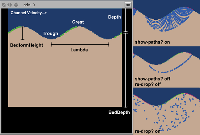
Figure 1. Parameter definitions and settings controlled by the user. In Interface, tracer particles are released in a flux-weighted manner at the water/sediment interface and tracked through the sediment. If show-paths? is “on” the water tracers mark where they have been, showing their paths. When a tracer returns to the surface water, this changes the total number of tracers in the system, when re-drop? is set to “off”. The cumulative residence time distribution plot shows this change by plotting the ratio of the number of tracers remaining in the sediment bed to the initial number as a function of time. If re-drop? is “on” then tracers that leave the system are replaced in the same flux-weighted manner as original particles, and the cumulative plot is disabled. Please click here to view a larger version of this figure.

Parameter Name	Units	Definition			Interface	Mousedrop
Lambda (λ)	cm	Wavelength of bedform (see Figure 1)
BedformHeight (H)	cm	Twice the bedform amplitude (see Figure 1)
BedDepth (D)	cm	Depth of the sediments (see Figure 1)
HydrCond (K)	cm/s	Hydraulic Conductivity
Porosity (θ)		Porosity
ChannelVelocity (U)	cm/s	Mean velocity in the surface water or channel
Depth (d)	cm	Water depth (see Figure 1)
Slope (S)		Slope of the bedforms and water surface
NumParticles		The number of particles released into the system.
TimeX (Time1, Time2..)	min	Time at which each color change occurs
Simulation Buttons		Definition			Interface	Mousedrop
Setup		Set’s up the simulation using parameters shown
go/stop		Starts and stops the simulation
Step		Clicking step causes one time step to pass.  This allows users to slow down the code and see exactly what happens in 100 sec.
clear paths		Clears all he blue particle paths from the screen
Advance to next time		This causes the program to run until the next color change time (TimeX)
mouse-drop		This button must be clicked before particles may be placed in the subsurface by clicking on locations in the subsurface.
show-paths?		If show-paths? is “on” the water particles leave a trail of blue showing where they have been (see Figure 1).
re-drop?		If re-drop? is “on” the particles are replaced in a flux weighted manner for every particle, which exits the system, and the cumulative plot does not work.  When a particle exits the hyporheic zone the number of particles in the system decreases if re-drop? is “off” (see Figure 1).

Table 1. Hyporheic Parameters and Simulation Controls. Each parameter, button, and slider that can be adjusted by the user is given in this table along with a definition.

In this simulation, two processes induce fluid velocity in the sand bed. The first is due to the interactions of the stream flow with bedforms. The velocity head at the water/sediment interface induced by bedforms is also approximately sinusoidal, and shifted by a quarter wavelength from the bedform itself²². The amplitude of the velocity head function at the surface-subsurface interface has been approximated from measurements as¹⁶:

Equation 2:

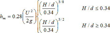
where U is the mean surface water velocity, g is the gravitational constant, and d is the depth of the water (shown in Figure 1). The velocity head function is then given by:

Equation 3:

This head function can then be used to calculate the bedform-based component of the subsurface velocity functions by solving the Laplace equation with a constant sand bed depth²⁰. The second component of the porewater velocity is determined by the slope of the system, S, which corresponds to a gravitational head gradient that yields flow in the downstream direction proportional to . The final functions for porewater velocity are:

Equation 4:

Equation 5:

where u is the longitudinal velocity component, v is the vertical velocity component, K is the average hydraulic conductivity of the sediment, is the average porosity of the sediments, y is the vertical coordinate, and D is the depth of the sediments.

Particle tracking simulations were created, which use the NetLogo modeling language and simulation platform²³. The two implementations (Mousedrop.nlogo and Interface.nlogo) use these equations to model hyporheic flow with the same simulation core. The primary difference is the initial locations of the tracer particles. Mousedrop allows the user to place simulated tracer anywhere within the subsurface. Subsurface velocity equations 4 and 5 are used to move the tracer to simulate dye injection experiments. In Interface, tracer is always placed along the surface/subsurface boundary in a flux-weighted manner. This mimics the delivery of dissolved and suspended material from the surface water into the porewater, which is crucial to understanding hyporheic exchange. The tracer then moves within the subsurface until it again reaches the stream water. Tracing the dye paths in the flume and simulating the paths using NetLogo yields the streamlines of the flowfield, as long as the flow conditions and bedform morphology remain steady during the period of observation. Interface.nlogo creates a cumulative residence time distribution, which shows the ratio of the number of tracer particles remaining in the sediments to the initial number of tracer particles placed at time 0 as a function of time.

As discussed in a recent literature survey²⁴, there remains considerable debate within the educational research community about the relative merits of hands-on laboratory experiments versus simulated labs and computer models. On the one hand, some feel that “hands-on experience is at the heart of learning”²⁵, and caution that cost-savings arguments may be fueling the replacement of hands-on lab activities by computer-based simulations, to the detriment of student understanding²⁶. On the other hand, some researchers in science/engineering education argue that simulations are at least as effective as traditional hands-on labs²⁷, or discuss the benefits of computer-simulation in fostering student-centered “discovery learning”²⁸. While consensus has not been reached, many researchers have concluded that, ideally, computer simulations should supplement, rather than supplant, hands-on laboratory experiments^29,30. There have also been initiatives within science and engineering education to simultaneously couple physical experimentation and real-world sensing with computer simulations of the phenomena; see, e.g., “bifocal modeling”³¹.

Students can gain a deeper conceptual knowledge and a better understanding of the scientific research process by interacting with both a physical system, and a computer-based simulation of that system. This procedure involves having students perform a solute transport experiment that demonstrates gravitational and bedform-induced hyporheic exchange flow, and match their own experimental setup and results with a computer simulation of the same phenomena. This comparison facilitates important student-learning outcomes, and a deeper discussion of the scientific method, and interplay between model/theory-building and empirical validation through data collection. After performing this comparison, students can also take advantage of the benefits of computer-based simulation to quickly explore a multitude of alternative scenarios by changing model parameters.

Protocol

1. Simulation Software

1. Use the software described in this section.
   1. Download and install the free/open-source multi-agent modeling language and simulation platform, NetLogo (Available: http://ccl.northwestern.edu/netlogo/, version 5.1 or later).
      Note: This software is available at no cost and runs on all major operating systems (Windows/Mac/Linux).
   2. Download the two specific simulation script files (mousedrop.nlogo and interface.nlogo) that accompany this laboratory procedure. (Available: http://modelingcommons.org/browse/one_model/4259 and http://modelingcommons.org/browse/one_model/4258)
      Note: Once the simulation platform is installed and these files have been downloaded, double-clicking these files automatically opens the simulations up, ready to run.

2. Flume Demonstration

1. Set up the laboratory flume so that all parameters (Table 1) fall within the mousedrop simulation parameter range constraints.
   Note: The constraints can be adjusted in mousedrop, if required for the physical system by editing the sliders.
   1. Pour a layer of approximately 15-25 cm of sand into the flume. Measure and record the hydraulic conductivity and porosity of the sand following standard methods^32,33.
   2. Fill the flume with approximately 20-30 cm of water.
   3. Start the flume and increase the flow rate to a level that is fast enough to move sand grains and thus to create bedforms.
      Note: The flow rate can be further adjusted to refine bedform characteristics with practice. Bedform sizes are a result of flow rate, water depth and sand properties.
   4. Allow bedforms to develop for 12-24 hr to form natural dune/ripple morphology. To accelerate this process, manually shape regular dunes, and then allow sediment transport for 4-12 hr. Alternatively, manually form regular triangular dunes.
      Note: Regular triangular dunes will yield regular patterns of hyporheic exchange, but will not show as much complexity as natural dune/ripple bedforms.
   5. Once the desired bedforms are achieved, reduce the water flow rate until bed sediment transport slows and bedform characteristics stop changing.
      1. Visually observe motion of sediment grains comprising the bed, and reduce flow until motion ceases.
         Note: This will preserve the bed morphology for the duration of the experiment.
      2. To confirm that slow, episodic motion is not occurring, mark or photograph bedform positions and then observe at a later time.
         Note: It is only important that bedforms do not move significantly over the time frame of the experiment, so that provides a sufficient observation time to confirm that bedforms are stable.
   6. Adjust flume slope and/or water depth to achieve uniform flow under the reduced flow rate.
      1. Control channel slope through equipment constructed into the flume, typically either a motorized jack or a hand-crank. Adjust water depth by adding or removing water from the flume.
         Note: In the experimental setup used here, the entire flume is mounted on a pivot on the downstream end, and the slope is set by a motorized jack at the upstream end.
      2. While the pump is running, select two longitudinal locations marked with lines perpendicular to the bottom of the flume. At these locations, use a ruler to measure the distance along these perpendicular lines, between the surface of the water and the bottom of the flume.
         Note: Depending on the flume setup, the bottom of the flume may serve as a better sloped reference line than the bottom of the flume. Selecting a larger longitudinal distance will yield greater accuracy.
      3. Adjust the slope of the flume and/or the water depth and re-measure until the vertical distance measurements are the same to achieve uniform flow. Measure the sloped horizontal distance along the bottom of the flume between these two longitudinal locations.
   7. Stop the pump and wait for the water to stop moving; this will provide a level surface. Re-measure the distance between the top of the flume and the water surface at each longitudinal location.
      Note: The channel slope is equal to the difference between these measurements, divided by the sloped horizontal distance between them.
   8. Re-start the pump.
   9. Select a test section, which should be a location near the middle or downstream end of the flume where dunes have formed a regular pattern. Ensure that this section encompasses at least one full bedform.
   10. Measure and record the average sediment depth (D) in the test section with any hand measuring devise (transparent rulers are ideal). For simplicity, use the average distance of a crest and trough to the flume bottom.
   11. Measure and record the average bedform height in the test section, defined as the difference between the sediment depth at a crest and the sediment depth at a trough with a ruler. Measure several bedforms to obtain a good estimate of the average.
   12. Again using the ruler, measure and record the average water depth (d) in the test section, defined as the average distance from the water surface to the sand bed. Again, use the average water depth at dune crests and troughs for simplicity.
   13. Record the channel flowrate (Q) from the flowmeter, and calculate the average velocity as Q / (d *w), where w is the width of the flume and d is the water depth.
       Note: Our flowmeter is inserted into the recirculation loop of the flume.
   14. Measure and record the average bedform wavelength in the test section. Typically, measure the wavelength as the distance between successive dune crests.
   15. Open the Mousedrop simulation (in the NetLogo platform) and check that all measurements are within the variable ranges specified in the simulation user interface. If a measured parameter falls outside of the constraint range, adjust the simulation parameter range by right-clicking on the parameter “slider”, selecting “edit”, and adjusting the min/max values.
2. Visualize hyporheic exchange.
   1. Set the camera in a fixed location (preferably on a tripod) pointed orthogonally to the flume wall with a single bedform in the test section centered in the picture.
      Note: This will avoid problems of slanted perspective.
   2. Take a test picture to verify conditions. Adjust the lighting if reflections are a problem.
   3. Using the syringe and needle, make 2-3 small dye injections near the flume wall. Ensure that these injections form ~2 cm round patches of colored porewater at a variety of vertical and horizontal locations. Use care to minimize the disturbance to the sand bed during the injection.
      Note: Injections of smaller volumes of dye allow the user see more detail and view individual stream paths.
   4. Record the start time of the dye injections and take an initial picture.
      Optional: It can be educational to trace the initial dye fronts with markers on transparency paper, so that the dye movement is easily observable in lab, but these outlines will also block small portions of the dye fronts in pictures, so there is a trade-off.
   5. Capture the dye front positions at appropriate time intervals. For time lapse photography, use 30 sec intervals to give smooth results.

3. Simulation

1. Run Simulation 1: Mousedrop and compare with observed dye transport.
   1. Open the simulation script named Mousedrop.nlogo.
      
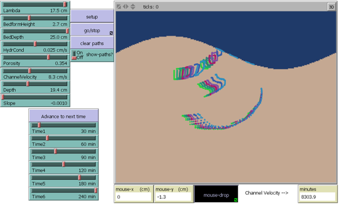
      Figure 2. Mousedrop. This shows where tracers are at 7 different instances in time. Please click here to view a larger version of this figure.
   2. Adjust the physical system parameters shown in Table 1 to match flume experimental conditions (specifically: Lambda, BedformHeight, BedDepth, HydrCond, Porosity, ChannelVelocity, Depth, and Slope). Be sure to pay careful attention to units when entering input parameters.
   3. Adjust sliders Time1, Time2, etc. to indicate times when the simulation tracking color will change. Set these color changes to match observation times in order to facilitate comparison of simulation results with observations.
      Note: If the Time parameters are all set to 0, the simulation will display a single color throughout.
   4. After all parameters are set, click the setup button.
      Note: The bedform should appear in the simulation view.
   5. Click the mouse-drop button to indicate the starting locations of virtual tracers. Note that multiple locations in the bed may be clicked. Hold the mouse down to release more virtual tracer. When simulating dye movement, use the mouse to either trace dye fronts (the boundary around the dye) or fill in the full area of the dyed region.
      Note: Introducing more virtual tracer will cause the simulation to run more slowly. The best visual results will vary with computer performance.
   6. Once all of the virtual tracers have been placed, you can either click the Advance to next time button, which will start the simulation and then stop it at the first time or you can click the go/stop button to begin the simulation indefinitely. Do not re-click the setup button, or the tracers will have to be placed again.
      Note: Once the simulation starts running, the velocity is calculated for the location of each tracer based on simulation parameters in Equations 4 and 5. The tracer moves according to the velocity field for 100 simulated seconds and then the velocity at the new location is calculated and the procedure is repeated until the tracer leaves the system.
   7. Optionally, click the go/stop button repeatedly to pause/continue the simulation. Compare the simulated and measured dye distributions at different points in time.
2. Run Simulation 2: Interface.
   1. Open the script titled Interface.
      
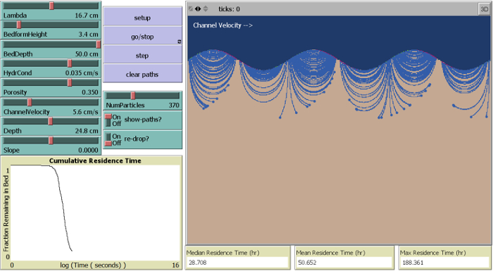
      Figure 3. Interface. This shows 370 tracers flowing through the subsurface using the interface simulation. The tracer paths show where each tracer has been since it was started at the surface water-subsurface interface. Eventually all flow paths should return to the surface water. Please click here to view a larger version of this figure.
      Note: This script introduces virtual tracers on the streambed surface in a flux-weighted manner based on calculated subsurface velocities. This provides a visual representation of the relative amounts of water flowing into (and out of) the streambed at different locations.
   2. Begin by clicking setup followed by go/stop.
      Note: This will run the simulation with the default settings. The re-drop? switch is initially set to off, so the cumulative residence time distribution will be plotted as time passes.
   3. After observing the simulation with the default parameters, click go/stop to stop the simulation.
   4. Change one or more parameters and then click setup followed by go/stop.
      Note: This will restart the simulation with the parameters that have been selected.

Results

The use of a simulation in conjunction with experiments allows students to observe the similarities and differences between idealized mathematical models and more complex real systems. Figure 4 shows an example comparing dye injection photographs with Mousedrop simulations. The initial photograph is used to determine the placement of the simulated dye tracer at time zero, and then the simulation is run for 34.2 min and compared with a photograph taken at that time. Overall the model does an exce...

Discussion

In conjunction, the flume demonstration and particle tracking simulations provide a comprehensive introduction to hyporheic flow for a range of audiences. Participants of all levels are provided visual evidence for the occurrence of hyporheic exchange induced by bedforms, and the strong variability in subsurface flow paths under bedforms. These procedures can be used as a simple demonstration of porewater flow for undergraduates or K-12 students, or it can be used in graduate courses in conjunction with a more in-depth p...

Materials

List of materials used in this article

Name	Company	Catalog Number	Comments
Flume	Engineering Laboratory Design	Custom	Laboratory flume with clear sides for 24-48 hours. Alternatively a small teaching flume can be constructed for under 300 dollars following the guidelines provided in our supplementary materials.
Flowmeter	Rosemount	8800 vortex	This is located inside the recirculation loop of the flume
Sand	US. Silica	F30	Research-grade sand to form a layer 10-20 cm deep throughout the flume
Dye	Samples from food companies		Water-soluble food grade dye made into an aqueous solution. Dark colors like red, blue and green work best. (Avoid food dyes in propylene glycol.)
Syringe	HSW	4100.000V0	5-10 ml, e.g. HSW Norm-Ject 2-part disposable syringe
Pipetting Needle	Cadence Science	7942	14-gage, 6-in blunt end,  to inject the dye deep into the sand.
Digital Camera	Any		Digital camera with steady tripod. (Time lapse cameras can be used to collect rapid evenly spaced data.) We used a Nikon D7000.
Ruler	Any		Transparent is best.
Measuring Tape	Any
Netlogo Software	CCL		http://ccl.northwestern.edu/netlogo/
Mousedrop.nlogo	Netlogo Commons	4259	http://modelingcommons.org/browse/one_model/4259
Interface.nlogo	Netlogo Commons	4258	http://modelingcommons.org/browse/one_model/4258