Blast Quantification Using Hopkinson Pressure Bars

Summary

This protocol details the use of Hopkinson pressure bars to measure reflected blast loading from near-field explosive events. It is capable of interpolating a pressure-time history at any point on a reflective boundary and as such can be used to fully characterize the spatial and temporal variations in loading produced.

Abstract

Near-field blast load measurement presents an issue to many sensor types as they must endure very aggressive environments and be able to measure pressures up to many hundreds of megapascals. In this respect the simplicity of the Hopkinson pressure bar has a major advantage in that while the measurement end of the Hopkinson bar can endure and be exposed to harsh conditions, the strain gauge mounted to the bar can be affixed some distance away. This allows protective housings to be utilized which protect the strain gauge but do not interfere with the measurement acquisition. The use of an array of pressure bars allows the pressure-time histories at discrete known points to be measured. This article also describes the interpolation routine used to derive pressure-time histories at un-instrumented locations on the plane of interest. Currently the technique has been used to measure loading from high explosives in free air and buried shallowly in various soils.

Introduction

Characterizing the output of explosive charges has many benefits, both military (defending against buried improvised explosive devices in current conflict zones) and civilian (designing structural components). In recent times this topic has received considerable attention. Much of the knowledge gathered has aimed at the quantification of the output from charges to enable the design of more effective protective structures. The main issue here is that if the measurements made are not of high fidelity then the mechanisms of load transfer in these explosive events remain unclear. This in turn leads to problems validating numerical models which rely on these measurements for validation.

The term near-field is used to describe blasts with scaled distances, Z, less than ~1 m/kg^1/3, where Z = R/W^1/3, R is the distance from the center of the explosive, and W is the charge mass expressed as an equivalent mass of TNT. In this regime the loading is typically characterized by extremely high magnitude, highly spatial and temporally non-uniform loads. Robust instrumentation is hence required to measure the extreme pressures associated with near-field loading. At scaled distances Z < 0.4 m/kg^1/3, direct measurements of the blast parameters are either non-existent or very few¹ and the semi-empirical predictive data for this range is based almost entirely on parametric studies. This involves using the semi-empirical predictions given by Kingery and Bulmash², which is outside of the author's intended scope. Whilst tools based on these predictions^3,4 allow for excellent first-order estimations of loading they do not fully capture the mechanics of near-field events, which are the focus of the current research.

Near-field blast measurements have in recent times focused on quantifying the output from buried charges. The methodologies employed vary from assessing the deformation caused to a structural target^5-7 to direct global impulse measurement^8-13. These methods provide valuable information for the validation of protective system designs but are not capable of fully investigating the mechanics of load transfer. Testing can be done at both laboratory scales (1/10 full scale), or at near to full scale (> 1/4), with pragmatic reasons such as controlling burial depth or ensuring no inherent shape of the shock front is generated by the use of detonators rather than bare charges¹⁴. With buried charges the soil conditions need to be highly controlled to guarantee the repeatability of the testing¹⁵.

Independent of the whether the charge is placed in free air or is buried, the most fundamental issue in measuring the resulting blast is ensuring the validity of measurements made by the instrumentation deployed. In the designed test apparatus¹⁶ a fixed 'rigid' target plate is used to shield the Hopkinson pressure bars¹⁷ (HPBs) whilst at the same time ensuring that the ends of the bars can only record the fully reflected pressures. The authors have previously shown that measurement of reflected pressure from a rigid target is more accurate and repeatable than incident, or 'free-field' measurements^18-20. The geometry of this plate is such that any pressure relief generated by clearing or flow around the target edge²¹ would be negligible. This new test apparatus has been constructed at 1/4 scale. At this scale tight control over the burial conditions and the explosives can be ensured, with the full scale charge size of 5 kg scaled down to 78 g, at a burial depth of 25 mm.

Protocol

1. Rigid Reaction Frame

1. Determine scaled distance at which testing will take place using Equation 1, where R is the distance from the center of the explosive, and W is the charge mass expressed as an equivalent mass of TNT.
   Z = R/W^1/3     (1)
2. Calculate approximate maximum impulse this arrangement will generate via numerical modelling (see Appendix A) or specific tools such as ConWep³.
   Note: The use of ConWep³ is only valid for free air blast, if an estimation of the pressures generated from buried charges is required the more advanced numerical modelling is required.
3. Check the estimated loading from the modelling will not generate in-plane displacements of more than 0.5 mm in the target plate.
4. Increase the loading calculated by a factor of 10 to account for inaccuracies in the modelling and to add flexibility for future testing.
5. Design a rigid reaction frame to be able to resist the maximum loading calculated¹⁶. In an Engineering department, perform these calculations in house; otherwise seek the services of a Structural Engineer.
   1. Procure rigid reaction frames, contract a specialist contractor to fabricate and install the frames to the designs of the structural engineer.
6. Procure target plate, contract a specialist steel fabricator.
   Note that the plate will need to be mounted on load cells (if used) and that holes for the HPBs (designed in section 3) will need to be drilled through the plate before mounting.

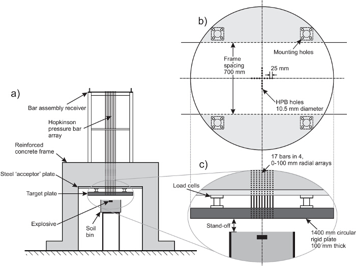
Figure 1. Schematic of the test frame. (A) Overall arrangement, (B) plan of target plate, (C) close-up view of target plate. The Hopkinson pressure bars are hung from the bar assembly receiver so that they sit flush with the face of the target plate. This allows the fully reflected pressure acting on the target plate to be recorded. Please click here to view a larger version of this figure.

2. Load Cell Design

1. Procure or fabricate load cells (if used). These can either be off-the-shelf universal (compression/tension) strain-gauge canister models or built in-house using sections of thick wall mild steel tubing welded to mounting plates with strain gauges affixed in a Wheatstone bridge formation as shown in Figure 2.
2. If the load cells have been fabricated in-house, send them to an external contractor for calibration.

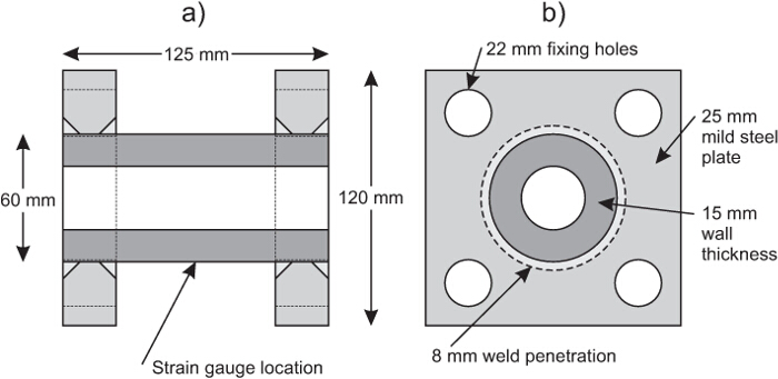
Figure 2. Diagram of the in-house fabricated load cells. (A) Side elevation, (B) end elevation. The dark grey cylinder is a thick wall steel tube which strains under loading. This strain is recorded using a single strain gauge as no rotation is experienced during the loading. From the calibration of the load cell the strain can be related back to the stress applied. Please click here to view a larger version of this figure.

3. Hopkinson Pressure Bar Design

1. Determine the duration of recording, , required to capture the full loading from the blast. The minimum duration required is the time taken in the numerical model (section 1.2) for the pressure to return to zero, after the initial pressure spike. Here, use 1.2 msec.
2. Decide on the material of choice for the HPBs. This affects the elastic wave speed, , in the bar which is given by where is the Young's modulus and is the density. For measuring a high pressure shock, use stiff materials such as steel; where as if a weaker shock is expected, use less stiff materials such as a magnesium alloy or even nylon.
3. Choose the position on the HPB that the strain gauge will be positioned, being as close as possible to the loaded face of the HPB to minimize dispersion. In the current set-up the thickness of the target plate and the manoeuvrability required to fit the bars in place meant that the gauges could only be installed 250 mm from the loaded face.
4. Calculate the HPB length required using , where is the distance from the loaded face of the HPB to the strain gauge and (3.25 m).
5. Determine required HPB radius to have sufficient bandwidth to capture the event using: kHz, where is the HPB radius in mm^22,23 (5 mm).
6. Decide on the spatial resolution required to capture the distribution of pressure across the plate. This is generally as close as possible while maintaining the structural integrity of the target plate. In the current work, use 25 mm.
7. Drill holes in the target plate to mount the HPBs (this can be part of the fabrication process). A close fit is required without the HPBs being in contact with the plate. Here, use 0.5 mm tolerance with 17 holes being drilled in a cross shape (Figure 1b).
8. Procure the HPBs (17), making sure to have the distal ends threaded to allow for suspension in the bar assembly receiver (Figure 3A).

4. Experimental Setup & Data Acquisition

Note: With the reaction frame, target plate, load cells and HPBs designed and fabricated, assembly can begin as shown in Figure 1, and designed in protocol section 1.

1. Attach semiconductor strain gauges to HPBs (Figure 3B) and load cells using cyanoacrylate, being careful to ensure continuity of earth through all cabling. An example of the Wheatstone bridge used for the HPBs is shown in Figure 3C.
   1. Verify all earth cables are attached to ensure continuity of earth. Well earthed test apparatus will improve signal quality notably.
2. Ensure wiring is sufficiently long to make sure the oscilloscope is locatable in a blast free area (shielded wiring should be used which has sufficient signal bandwidth).
3. Fit the target plate to the rigid reaction frame, using the optional load cells if present (Figure 1C).
4. Hang HBPs from the bar assembly receiver, passing the loaded end through the correct hole in the target plate. Hang the HPBs freely from a nut screwed onto the threaded distal end of the HPB.
5. Ensure bars are vertical using a spirit level (adjusting the receiver accordingly).
6. Check the faces of the HPBs are level with the target plate, adjusting the nut accordingly.
7. Set the trim on the variable resistor in the conditioning circuit (Figure 3C) to keep voltage within the limits of oscilloscope during testing. Do this through trial and error aiming to set the out of balance for each channel as seen on the digital readout on the amplifier boxes to zero.
8. Connect the amplified gauge output to a suitable digital oscilloscope. Configure to have a sampling frequency (1.56 MHz), recording duration (28.7 msec) with a pre-trigger duration of 3.3 msec.
   1. Set the recording to trigger when the voltage in the break wire channel (which is itself wired into the oscilloscope) exceeds an 'out-window'. Record voltage for each gauge connected (22 in total, 17 HPBs, 4 load cells and the break wire) and time.

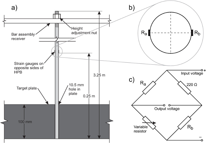
Figure 3. (A) Diagram of a HPB fitted into the target plate, (B) section through HPB at gauge location, (C) example Wheatstone bridge circuit. Two strain gauges are used in the Wheatstone bridge so that and bending of the Hopkinson bar is cancelled out. Please click here to view a larger version of this figure.

5. Explosive preparation

1. Decide on the explosive charge mass and stand-off to be used in the tests (100 g PE4 at 75 mm).
2. Decide whether the charges are to be detonated in free air or within another medium (soil, water etc.). For free air tests a spherical charge shape is normally utilized whereas with buried charges the standard is a 3:1 squat cylinder^24,25.
3. For free air tests:
   1. Suspend the charge below the target plate at the correct stand-off (75 mm). Achieve this with a thin timber strip or by placing the charge on a sheet of polythene.
   2. Place the charge co-axially with the measurement array to ensure valid readings.
   3. For free air tests use an electrical detonator, with the detonator being placed half way into the charge from the base. Do this at the last moment before firing and when the range has already been made safe.
4. For buried tests:
   1. Fabricate a suitable container for the medium. For soils, the current testing uses 1/4 scale containers²³.
   2. Decide upon the soil type to be utilized and the geotechnical conditions: moisture content and dry density of the soil, see ref.¹⁵ for more details.
   3. Decide on the burial depth to use in the testing. This is usually 100 mm in a full scale test, as the current tests are done at ¼ scale this means a 25 mm burial depth.
   4. Mix the soil thoroughly using a suitably sized construction mixer to achieve the target moisture content. For sands the mixing time required is 10 min.
      1. Check the moisture content of the mix by removing a small amount and weigh it to calculate the total mass, . Dry the removed soil and re-weigh to calculate the mass of water, . Geotechnical moisture contents are specified in terms of gravimetric moisture content, .
      2. If the moisture content is within tolerance continue, otherwise remix the soil. A tolerance of ±0.05-0.1% has been achieved in the current work.
   5. Weigh the empty soil container and calculate the volume to enable calculation of the soil density once full (step 5.4.7).
   6. Compact the soil in layers, thin enough to guarantee the target density, ensuring that the mass of soil entering the container is known. For Leighton Buzzard Sand¹⁵ this is done in two layers.
   7. Once the container is full, check that the density of the soil within is in tolerance (±0.2%). The target dry density in all tests with Leighton Buzzard Sand was 1.6 Mg/m³. Calculate dry density, using , where ρ_d is the dry density, M is the total mass of soil added to the container, V is the volume of the soil container and w is the moisture content.
   8. Excavate a small hole ≈50 mm to allow the charge to be placed with the top surface at the correct burial depth (25 mm).
   9. Place a non-electrical detonator into the base of the charge, and excavate a suitable channel to the side of the container to ensure the top surface of the container is uninterrupted once the soil is replaced.
   10. Place charge and detonator into the excavated hole, checking the burial depth is correct. Back fill the hole with the excavated material.

6. Firing sequence

Note: there is a small amount of overlap with protocol section 5 due to the nature of the testing. The firing sequence should aim to minimize risk and should only be conducted by suitably trained staff.

1. For free air tests:
   1. Arrange charge support below the target plate at the correct stand-off (75 mm).
   2. Close the range. Deploy sentries to ensure range is clear during firing.
   3. Place charge on the support co-axial to the instrumentation. Attach the break wire to the detonator, and place the detonator in the charge.
2. For buried tests:
   1. Place soil container so that the charge is placed co-axial to HPB array.
   2. Close the range. Deploy sentries to ensure range is clear during firing.
   3. Connect the break wire, ensuring it is wrapped around the periphery of charge (this gives a more repeatable time of detonation in buried charges).
3. Move to firing point and confirm instrumentation is running.
4. Supply power to the break wire. Check with sentries it is safe to proceed with the firing.
5. Initiate explosives. Make the test area safe.
6. Download and back up data.
7. Re-open test range.

7. Numerical interpolation for a 1D HPB array

1. Import the data from the raw data files into Matlab.
2. Time-shift all data in the radial direction so that the peak pressure for each bar arrives at the same time as the peak pressure of the central bar using Equation 2 (Figure 4B).
        (2)
3. Interpolate the pressure at any radial distance from Figure 4B.
4. Plot the arrival times () used to align the peak pressures and fit a cubic equation through the data (Figure 4C).
5. Time-shift the interpolated data to fit the arrival times, generating a continuous shock front (Figure 4D).
6. Repeat for each individual set of test data.

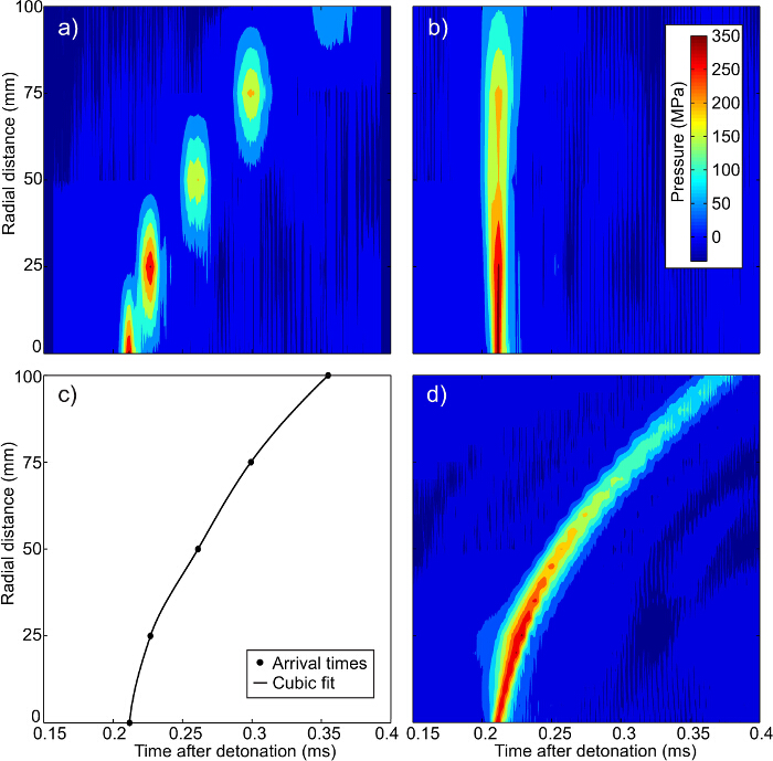
Figure 4. Interpolation sequence for 1D HPB array. (A) Original data, (B) time-shifted data, (C) shock front arrival times, and (D) final interpolated pressure time data¹⁶. The discrete nature of the pressure time histories can clearly be seen in (A) with there being no continuity between the peak pressures at each of the five gauge locations. When aligned by peak pressure as in (B) the interpolation of pressure at any radial distance (assuming the same arrival time) is possible. By recording the time shift required to align the peak pressures the arrival time of the shock front can be calculated as shown in (C). This then allows the arrival time and pressure time history to be calculated for any radial distance be interpolation of pressure from (B) and time from (C) giving the final interpolated pressure as seen in (D). Please click here to view a larger version of this figure.

8. Numerical interpolation for a 2D HPB array

Note: The code used to run the interpolation in Matlab has been provided along with an example results file which will be referred to in this section.

1. Import the data from the raw data files into Matlab. For the example test data, double click on the test_data.mat file, and then click 'Finish' in the Import Wizard.
2. Open the interpolation2d.m Matlab script.
3. Define a regular grid over which the interpolation will run by changing the mesh. Ensure this is the same resolution as the mesh in any future numerical modelling^26,27. This is set in the '%mesh details' section of the code.
4. Run the interpolation2d.m Matlab script. Note the following steps are implemented in the code and are listed here for clarity.
   1. Time-shift all HPB pressure traces by (Equation 2). Original data is shown for mm in Figure 5B, with the same data time-shifted in Figure 5C.
      Note: The time shift is required to allow the interpolation routine to successfully locate the shock front at any given time. This essentially involves aligning the data for each radial array so all the maximum pressures align.
   2. Calculate the radius, , and angle, for a given point of interest on the grid, as shown in Figure 5A.
   3. Apply the 1D interpolation to the two HPB arrays closest to the point of interest for the current radius (for the interpolation would use the and  arrays).
   4. Interpolate linearly between the 2 pressures based on (again for a the weighting would be 50% of the and 50% of the array calculated pressures).
   5. Calculate the instantaneous load by multiplying the interpolated pressure by the grid spacing (area) to give the load.
   6. Multiply the load by the time step of the sampling to obtain the instantaneous impulse.
   7. Repeat for all locations and times (summing the instantaneous impulse to give the total impulse).
   8. Time-shift the pressure time history for each location based on cubic interpolation of the shock arrival time (Figure 5D).

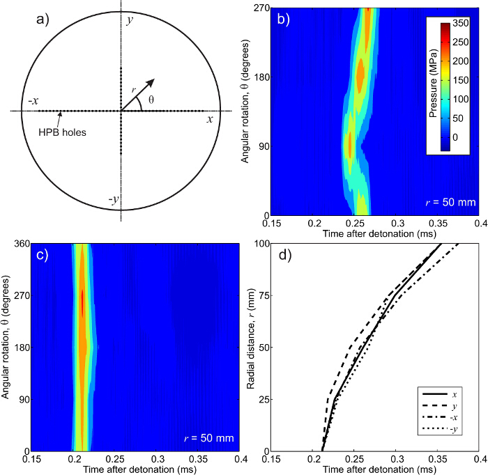
Figure 5. Interpolation sequence for 2D HPB array. (A) Sign conventions used, (B) original data mm, (C) time-shifted data mm, and (D) arrival times for each radial direction¹⁶. For a 2D array of bars the pressure time history at any point is dependent on both radial distance and which quadrant the point of interest is located. If the blast were perfectly symmetric then the pressures in (B) would form vertical lines as shown in (C). In (B) it can be seen that the shock front is reaches the 50 mm location on  axis first.
Please click here to view a larger version of this figure.

Results

An effectively rigid reaction frame needs to be provided. In the current testing a total imparted impulse of several hundred Newton-seconds needs to be resisted with minimal deflection. An illustration of the rigid reaction frame used is given in Figure 1. In each frame a 50 mm steel 'acceptor' plate has been cast into the base of the cross beams. Whilst not explicitly required, this allows for easy fixing of the load cells / target plate and provides added protection to ...

Discussion

Using the protocol outlined above the authors have shown that it is possible to get high fidelity measurements of the highly varying loading from an explosive charge, using an array of Hopkinson pressure bars. Using the interpolation routine outlined the discrete pressure-time histories can be transformed into a continuous shock front which is usable directly as the loading function in numerical modelling or as validation data for the output of such models.

When using buried charges the method...

Materials

List of materials used in this article

Name	Company	Catalog Number	Comments
Load Cell	RDP	RSL0960	This is only indicative, the exact load cell should be able to resolve the required loading
Steel target plate / HPBs	Garratts		Fabricated to order
Strain gauge	Kyowa	KSP-2-120-E4	To use with steel HPBs
Cyanoacrylate	Kyowa	CC-33-A	Check with manufacturer depending on mar material to be used
Digital Oscilloscope	TiePie	HS4 16-bit Handyscopes	6 used in parallel in current testing
Leighton Buzzard sand	Garside sands	Garside 14/25	Uniform silica sand

References

- Esparza, E. Blast measurements and equivalency for spherical charges at small scaled distances. Int. J. Impact Eng. 4 (1), 23-40 (1986).
- Kingery, C. N., Bulmash, G. ARBRL-TR-02555. Airblast parameters from TNT spherical air burst and hemispherical surface burst. , U.S Army BRL. Aberdeen Proving Ground, MD, USA. (1984).
- Hyde, D. W. Conventional weapons program (ConWep). , U.S Army Waterways Experimental Station. Vicksburg, MS, USA. (1991).
- Randers-Pehrson, G., Bannister, K. A. ARL-TR-1310. Airblast loading model for DYNA2D and DYNA3D. , U.S Army Research Laboratory. Aberdeen Proving Ground, MD, USA. (1997).
- Neuberger, A., Peles, S., Rittel, D. Scaling the response of circular plates subjected to large and close-range spherical explosions. Part II: Buried charges. Int. J. Impact Eng. 34 (5), 874-882 (2007).
- Xu, S., et al. An inverse approach for pressure load identification. Int. J. Impact Eng. 37 (7), 865-877 (2010).
- Pickering, E. G., Chung Kim Yuen, S., Nurick, G. N., Haw, P. The response of quadrangular plates to buried charges. Int. J. Impact Eng. 49, 103-114 (2012).
- Bergeron, D. M., Trembley, J. E. Canadian research to characterize mine blast output. 16'th Int. Symp. on the Military Aspects of Blast and Shock, Oxford, UK, , (2000).
- Hlady, S. L. Effect of soil parameters on landmine blast. 18'th Int. Symp. on the Military Aspects of Blast and Shock, Bad Reichenhall, Germany, , (2004).
- Fourney, W. L., Leiste, U., Bonenberger, R., Goodings, D. J. Mechanism of loading on plates due to explosive detonation. Int. J. on Blasting and Fragmentation. 9 (4), 205-217 (2005).
- Anderson, C. E., Behner, T., Weiss, C. E. Mine blast loading experiments. Int. J. Impact Eng. 38 (8-9), 697-706 (2011).
- Fox, D. M., et al. The response of small scale rigid targets to shallow buried explosive detonations. Int. J. Impact Eng. 38 (11), 882-891 (2011).
- Ehrgott, J. Q., Rhett, R. G., Akers, S. A., Rickman, D. D. Design and fabrication of an impulse measurement device to quantify the blast environment from a near-surface detonation in soil. Experimental Techniques. 35 (3), 51-62 (2011).
- Pope, D. J., Tyas, A. Use of hydrocode modelling techniques to predict loading parameters from free air hemispherical explosive charges. 1st Asia-Pacific Conference on Protection of Structures Against Hazards, Singapore, , (2002).
- Clarke, S. D., et al. Repeatability of buried charge testing. 23rd Int. Symp. on the Military Aspects of Blast and Shock, Oxford, UK, , (2014).
- Clarke, S. D., et al. A large scale experimental approach to the measurement of spatially and temporally localised loading from the detonation of shallow-buried explosives. Meas Sci Technol. 26, 015001(2015).
- Hopkinson, B. A Method of Measuring the Pressure Produced in the Detonation of High Explosives or by the Impact of Bullets. Philos. Trans. R. Soc. (London) A. 213, 437-456 (1914).
- Rigby, S. E., Tyas, A., Fay, S. D., Clarke, S. D., Warren, J. A. Validation of semi-empirical blast pressure predictions for far field explosions - is there inherent variability in blast wave parameters?. 6th Int. Conf. on Protection of Structures against Hazards, Tianjin, China, , (2014).
- Rigby, S. E., Tyas, A., Bennett, T., Clarke, S. D., Fay, S. D. The negative phase of the blast load. Int. J. of Protective Structures. 5 (1), 1-20 (2014).
- Rigby, S. E., Fay, S. D., Tyas, A., Warren, J. A., Clarke, S. D. Angle of incidence effects on far-field positive and negative phase blast parameters. Int. J. of Protective Structures. 6 (1), 23-42 (2015).
- Tyas, A., Warren, J., Bennett, T., Fay, S. Prediction of clearing effects in far-field blast loading of finite targets. Shock Waves. 21 (2), 111-119 (2011).
- Tyas, A., Watson, A. J. A study of the effect of spatial variation of load in the pressure bar. Meas Sci Technol. 11 (11), 1539-1551 (2000).
- Tyas, A., Watson, A. J. An investigation of frequency domain dispersion correction of pressure bar signals. Int. J. Impact Eng. 25 (1), 87-101 (2001).
- NATO Standardisation Agency. Procedures for evaluating the protection level of logistic and light armoured vehicles. Allied Engineering Publication (AEP) 55. 2, 2, (2011).
- Elgy, I. D., et al. UK ministry of defence technical authority instructions for testing the protection level of vehicles against buried blast mines. , Defence Science and Technology Laboratory. UK. (2014).
- Clarke, S. D., et al. Finite element simulation of plates under non-uniform blast loads using a point-load method: Buried explosives. 11th Int. Conf. on Shock & Impact Loads on Structures (SILOS), Ottawa, Canada, , (2015).
- Rigby, S. E., et al. Finite element simulation of plates under non-uniform blast loads using a point-load method: Blast wave clearing. 11th Int. Conf. on Shock & Impact Loads on Structures (SILOS), Ottawa, Canada, , (2015).
- Hallquist, J. O. LS-DYNA theory manual. Livermore Software Technology Corporation, CA, USA, , (2006).
- Fay, S. D., et al. Capturing the spatial and temporal variations in impulse from shallow buried charges. 15th Int. Symp. on the Interaction of the Effects of Munitions with Structures (ISIEMS, Potsdam, Germany, , (2013).
- Fay, S. D., et al. Measuring the spatial and temporal pressure variation from buried charges. 23rd Int. Symp. on the Military Aspects of Blast and Shock, Oxford, UK, , (2014).
Access restricted. Please log in or start a trial to view this content.
Reprints and Permissions