Experimental Methodology for Estimation of Local Heat Fluxes and Burning Rates in Steady Laminar Boundary Layer Diffusion Flames

Summary

We describe the use of micro-thermocouples to estimate local temperature gradients in steady laminar boundary layer diffusion flames. By extension of the Reynolds Analogy, local temperature gradients can be further used to estimate the local mass burning rates and heat fluxes in such flames with high accuracy.

Abstract

Modeling the realistic burning behavior of condensed-phase fuels has remained out of reach, in part because of an inability to resolve the complex interactions occurring at the interface between gas-phase flames and condensed-phase fuels. The current research provides a technique to explore the dynamic relationship between a combustible condensed fuel surface and gas-phase flames in laminar boundary layers. Experiments have previously been conducted in both forced and free convective environments over both solid and liquid fuels. A unique methodology, based on the Reynolds Analogy, was used to estimate local mass burning rates and flame heat fluxes for these laminar boundary layer diffusion flames utilizing local temperature gradients at the fuel surface. Local mass burning rates and convective and radiative heat feedback from the flames were measured in both the pyrolysis and plume regions by using temperature gradients mapped near the wall by a two-axis traverse system. These experiments are time-consuming and can be challenging to design as the condensed fuel surface burns steadily for only a limited period of time following ignition. The temperature profiles near the fuel surface need to be mapped during steady burning of a condensed fuel surface at a very high spatial resolution in order to capture reasonable estimates of local temperature gradients. Careful corrections for radiative heat losses from the thermocouples are also essential for accurate measurements. For these reasons, the whole experimental setup needs to be automated with a computer-controlled traverse mechanism, eliminating most errors due to positioning of a micro-thermocouple. An outline of steps to reproducibly capture near-wall temperature gradients and use them to assess local burning rates and heat fluxes is provided.

Introduction

While critical advancements have been made in the area of fire safety research over the past century, predicting rates of flame spread still remains a challenge for many materials in diverse configurations. Flame spread often proceeds in either the built or natural environments as a series of ignitions of new elements, emanating from an initial source of ignition. Knowledge of the burning characteristics of individual burning materials is critical in order to predict these rates of flame spread, because this contributes to rates of heating to unignited elements. The heat-release rate (HRR) of a fuel element has therefore been cited as the most fundamental quantity in fire research¹, being approximately equal to the burning (mass-loss) rate of the condensed-phase fuel, namely the evaporation rate of a liquid fuel or pyrolysis rate of a solid fuel.

The burning rate can be thought of as a measure of the flammability of a material and is a critical parameter in fire risk analysis and the design of fire suppression systems. The local mass loss (or burning) rate, ṁ"_f, of a vertical wall is, in particular, an important variable in many fire-related problems, such as flame spread on a wall, fire growth, and energy-release rates within an enclosure fire, and the spread of smoke and hot gas plumes. For prediction of upward flame spread on a vertical wall, the flame height must be calculated, which depends on the total energy release rate; that, in turn, is directly influenced by the local mass-loss rate integrated over the entire pyrolyzing area of the wall^2-3. While knowledge of these integrated mass-loss rates are relatively well known, knowledge of mass-burning rates at incremental locations along a fuel surface are not well known because experimental techniques to measure such rates are extremely limited. A technique that provides this "local" mass-burning rate information could provide increased insight to the burning of condensed fuels, enabling researchers to further understand the mechanisms which distinguish different fuels or configurations from one another. As most materials are first evaluated at the small scale (e.g., in a cone calorimeter¹), a logical first step is to provide a technique to measure local mass burning rates in small, laminar diffusion flames over condensed fuel surfaces.

The work presented here discusses the experimental methodology and protocols for carrying out experiments on steady laminar flames established over condensed fuel surfaces. Estimation of local temperature gradients using micro thermocouples is a particularly useful technique for the estimation of local mass burning rates and heat fluxes in these flames^4-6. An analysis of literature data shows the difficulty of determining local heat transfer, combustion and friction coefficients at the condensed fuel surface, which are important for understanding the physics and the underlying mechanisms that drive a particular fire and its spread^4-6. Components of heat fluxes, which have remained perhaps the most well-measured fire property at local locations over a fuel surface, have proved difficult to measure. Effects such as variability of fuels, heat flux scalability, difficulty of achieving steady state conditions and differing heat flux gauge technologies have contributed to a rather wide scatter of data which is available in the literature⁴. Measurements of local temperature gradients with high accuracy will help to alleviate this variability and also provide heat transfer correlations that could be used for numerical validation of laminar wall fires, a canonical fire research problem. Such experiments are also useful in exploring the dynamic relationship between a combustible condensed fuel surface and gas-phase flames in laminar and turbulent boundary layers. Methods to accurately capture these temperature gradients in an accurate and repeatable manner are described below.

Protocol

1. Planning of Experiments

1. Follow instructions and safety precautions before entering the fire or combustion research laboratory. Safety training is generally required for new users.
2. Schedule your experiments in advance to carry out the required tests. Consider the details of the experiment, transport of required fuels and necessary equipment.
3. Identify the liquid or solid fuel experiments of interest. Prepare the materials accordingly.

2. Preparation of Materials and Instrumentation

1. For liquid fuel experiments, prepare a fuel wick of porous noncombustible material (alkaline earth silicate wool). Previous experiments^4-6 have utilized 8 cm x 8 cm x 1.27 cm for free convection tests and 10 cm x 10 cm x 1.27 cm thick sheets for forced convection tests.
   1. Bake the given fuel wick for approximately 20 min by exposing it to a diffusion flame from a propane torch in order to burn organic binders inside the wick.
   2. In order to eliminate leakage of the liquid fuel from the sides of the wick, liberally apply liquid sodium silicate with a syringe covering all faces of the wick except the top face.
   3. Shield all but the top face of the wick with aluminum foil. Use a high temperature adhesive to paste the aluminum foil to the sides of the wick.
2. For solid fuel experiments, cut out a sheet of the solid fuel. In previous free convection experiments², an 8 cm x 8 cm x 1.27 cm thick sheet of a clear cast polymethyl methacrylate (PMMA) has been used.
3. Cut out a slot in a sheet of ceramic fiber insulation board equal to the size of the fuel sample in which to later mount the sample. Often, use the same porous noncombustible as the fuel wick; however seal it with high temperature matte black paint.
4. Check the given data acquisition hardware and software. Open the software and check the temperature mapping algorithm before carrying out required tests.

3. Preparation of the Experimental Setup

1. Place a side-view digital SLR camera so that it is aligned with the central axis of the fuel and far enough away so that the full side view of the given flame is captured.
   1. For forced-convection flames, image a field of view at the center of the fuel specimen covering an area of 16 cm x 8 cm for calculating the flame stand-off distance in the pyrolysis zone.
2. Place the traverse mechanism above the fuel sample. Attach a 50 µm wire-diameter micro thermocouple to the horizontal axis of the traverse mechanism with care.
3. Turn on the programmable stepper motor controller.
4. In the case of forced flow experiments, power up the centrifugal blower of the wind tunnel.
5. Set the pulse-width-modulation (PWM) controller to a frequency of 7,000 Hz with power settings ranging from 16% to 50% for different blower speeds, verified with a hot-wire anemometer.
6. Wear safety glasses and fire-resistant hand gloves before proceeding with the test.
7. During each test, soak the wick with liquid fuel (methanol or ethanol) up to its point of saturation. For an 8 cm x 8 cm x 1.27 cm thick wick, 90 ml was sufficient to fully soak the wick using two 60 ml syringes while for a 10 cm x 10 cm x 1.27 cm thick wick, 120 ml was found to be sufficient.
8. Place the fuel-soaked wick / solid fuel plate carefully into the fuel-wick holder. Check the flatness of the fuel wick surface with an angle gauge.
9. Open mass balance software and check the USB-interface settings. Check the mass balance and note its reading before the test.

4. Running Experiments in a Combustion or Fire Lab

1. Ensure proper ventilation of the experimental facility by turning on the exhaust after completing each set of experiments. Exhaust should be as minimal or isolated as possible during the experiments to help eliminate flow disturbances.
2. Before a sample is ignited, calibrate the side-view digital camera by taking a picture of a sheet of graph paper or ruler that is aligned along the central axis of the fuel surface. Obtain an average pixel/mm count from the calibration images. Use this value of pixels/mm during the post-processing of the images (for setting up the measurement scale in ImageJ).
3. Ignite the fuel with a propane torch, momentarily touching it for a liquid fuel wick and passing the flame uniformly over the surface for 50-60 sec with a solid fuel.
4. Start experimental time immediately after uniform ignition. Use a stop watch to denote the burning time.
5. Press the data acquisition button on the mass balance software.
6. Monitor the mass loss of the burning wick over a timed interval and write it to a measurement file. Use the mass balance software for the given purpose.
7. Repeat steps 4.3 to 4.6 for multiple tests under the same conditions to ensure repeatability.
8. Use the mass-loss versus time curve to determine the steady burning regime, where a linear fit of the mass loss has a high R² value.
9. For unsteady solid fuels, burn samples at 50 sec increments from ignition to burnout to measure surface regression (e.g., for 50 sec, 100 sec, 150 sec, etc.).
10. Cut burned solid fuels along the centerline after cooling for regression testing.
11. Take side-view photographs of cut solid fuels and load into ImageJ. Measure the regression at streamwise locations by converting pixels to cm with a ruler. Step by step procedure to process a given image in ImageJ is listed hereunder.
    1. Open side-view photograph of the solid fuel sample in ImageJ via Select File → Open Image.
    2. Open the calibration image (with ruler) of the solid fuel sample in ImageJ via Select File → Open Calibration Image.
    3. Stack up the calibration image and solid fuel sample image. Go to Image → Stacks → Images to stack.
    4. Set measurement scale: Draw a line between two points of known distance such as a ruler on the photograph. Go to Analyze → Set Scale. In the Set Scale window the length of the line, in pixels, will be displayed. Type the known distance and units of measure in the appropriate boxes and click OK.
    5. Draw a new line and confirm that the measurement scale is correct.
    6. Measuring distance between two points in the given sample photograph: Draw a line between two points. The status bar will show the angle (from horizontal) and the length. Analyze → Measure (or Ctrl+M or simply type M on the keyboard) transfers the values to a data window.
    7. Measure the regression at each streamwise location x by measuring the thickness of the burn-out sample and subtracting it from the initial thickness of the sample.
12. Note the time interval over which the surface of solid fuels remain approximately flat and use for temperature mapping, or adjustments of thermocouple positions made to compensate for surface regression.
13. Set the temperature mapping interval to capture measurements during the steady burning regime, approximately 150 sec for solid PMMA and 400 sec for liquid-soaked wicks. Set the temperature mapping interval based on the steady burning time interval of liquid and solid fuels. A recommended step size near the surface is 0.25 mm^4-6.
14. Align a micro thermocouple carefully with the surface of the fuel using a X-Y unislide. Place the given thermocouple at the center of width of the sample.
15. Move the micro thermocouple carefully to the leading edge of the fuel wick using the X-Y unislide.
16. Run a data acquisition program on a computer and read the grid scanning algorithm from a folder on the desktop.
    Note: Once the experiment is under way, data collection is automatic, and the user only needs to oversee it to make sure the experiment is going as planned.
17. Using a data acquisition program on a computer, acquire data and write it to a measurement file. Note, sampling rates of 100^4-5 to 500⁶ Hz were used in past experiments.
18. When finished, extinguish the flame. Turn off the PWM controller and disconnect the power plug of the blower from the 3-phase 240 VAC power outlet.
19. Turn off the stepper motor controller.
20. Repeat steps 4.12 to 4.18 for additional experiments at similar or different flow conditions with the same thermocouple. A minimum of 5 tests should be repeated for each given flow condition (e.g., forced flow velocity or vertical orientation).
21. Repeat steps 4.12 to 4.18 for a 75 µm micro thermocouple. Traverse two thermocouples (50 µm and 75 µm wire-diameter) along the same path at the center of the flame for accurate radiation corrections. Smaller thermocouples might also be used, however breakage often occurred for wires below 50 µm.

5. Data Analysis

1. Read the processed data from the LVM file into Matlab or other analytic software.
2. Average the temperature data at each spatial point from different tests.
3. Calculate a radiation correction from averaged thermocouple data at each streamwise location, following the correlation of Collis and Williams¹⁰ described in detail below.
4. Calculate compensated temperature measurements by adding the radiation correction to raw temperature data.
5. Non-dimensionalize the temperature data and spatial location.
6. Fit the non-dimensional temperature data at the fuel surface with an appropriate higher-order polynomial fit using a curve fit algorithm in Matlab or other dedicated software. 4 to 6 points near the surface were found to work well in previous studies^4-6.
7. Calculate the normal non-dimensional temperature gradients at the fuel surface from the slope of the higher order polynomial fit to the non-dimensional temperature distribution at the fuel surface (y=0).
8. Calculate the local mass burning rate from the corresponding local non-dimensional temperature gradient at the fuel surface using a theoretical correlation based on the Reynolds Analogy⁴.
9. Calculate the convective heat flux from the temperature gradient at the surface of the fuel^5-6.

Results

Experiments have been performed both in a vertical configuration and a unique horizontal wind tunnel facility at the University of Maryland, shown in Figure 1. Rather than a traditional pull or closed return wind tunnel, the wind tunnel facility at the University of Maryland uses a variable speed blower to pressurize a 100 x 75 x 100 cm plenum which drives the flow of air out a duct at the opposite end. This configuration enables continuous combustion experiments as smoke is not re-circulated, the wind tunnel is not damaged or influenced by the fire and thermocouples are able to freely move throughout the sampling section. The exit duct consists of a 122 cm, 30.5 cm wide converging section connected to the plenum. To straighten the flow and reduce the incoming turbulence intensity, fine mesh screens are placed at the entrance and exit of the converging section and a 5 cm thick honeycomb with 0.3 cm holes is placed 110 cm upstream from the tunnel exit. The velocity of the flow exiting the wind tunnel is controlled by varying the speed of the fan with a pulse-width-modulation (PWM) controller and fuel samples are placed at the outlet of the tunnel, where flow velocities have been checked via the use of a hotwire anemometer.

Fuel samples at the outlet of the wind tunnel were placed on top of a load cell which continuously measures the mass-loss of the sample over time. To avoid disturbances of the wind to the load cell, the sample was elevated on a sheet of aluminum (30.5 x 61.0 cm x 1.5 mm thick) by two U-brackets and surrounded by 1.27 cm thick ceramic fiber insulation board to ensure a smooth surface around the burning sample. The top surface of the board was coated with a high temperature black matte paint with an emissivity approximately 98% to ensure a good backdrop for visually observing the flame and to seal the insulation which also contains organic binders. Because the insulation board presents a relatively blunt body to the incoming flow, placing the sample setup directly in the outlet of the wind tunnel resulted in flow separation and significant turbulence observed in flames. Previous work by Ha et al. found that attaching an extension plate to the leading section of a fuel sample prevented this flow separation and ensured a laminar flow profile incoming to the sample. A 10 cm wide, 40.6 cm long thin, metal lip was therefore mounted from the leading edge of the sample to the outlet of the wind tunnel, providing a laminar diffusion flame that eventually was found to match existing theory⁷.

In testing liquid fuels a porous noncombustible wick was needed. A 10 cm x 10 cm x 1.27 cm thick sheet of Alkaline earth silicate wool was selected for forced flow experiments due to its high porosity and low thermal conductivity. In order to prevent leakage of fuel from the sample, sodium silicate glue was used to apply aluminum foil to all except the front face. The sample was also "baked' to remove organic binders by passing a blowtorch over the sample for approximately 20 minutes, at which point the flame changed from yellow to blue (indicating the removal of binders from the sample). During testing, wicks were soaked with approximately 120 ml of liquid fuel (ethanol or methanol) which was found to be the point of saturation for the 10 cm wide wicks.

The mass burning rate of the fuel was determined by measuring the mass lost from the sample over time during combustion at a rate of 1 Hz. The sample setup was supported over a precision mass balance with a maximum capacity of 32.2 kg and resolution of 0.1 g, fine enough to measure this mass-loss rate with high precision. Following ignition of the sample by a blowtorch, the mass-loss rate of the condensed fuel increases as a function of time, eventually reaching a constant rate which eventually fades toward the end of the test as the fuel burns out. This "steady" region, where evaporation of the fuel rather than diffusion through the wick dominates burning, is the region of interest where data is sampled. For a liquid wick, samples were found to burn with a steady mass-loss rate for approximately 400 sec, approximately the middle 80% of a test. All burning rates presented are averages of at least six repeated tests under specified conditions, where the repeatability of measurements were found to be within 1.2% of the mean.

For testing of a solid fuel sample, polymethyl methacrylate (PMMA) was selected as it burns relatively steadily and does not char. In order to ignite the sample, a blowtorch was passed over the sample surface for 50-60 sec, at which point the entire surface was uniformly ignited. Because the fuel sample was small and the experimental results found to be very repeatable, the method was deemed to be sufficient for ignition. Unlike liquid fuels soaked into a noncombustible wick, solid fuels regress as a function of time and are therefore never truly achieve a steady regime. Instead, early times of burning were chosen to be sampled where the fuel remained relatively flat, experimentally determined to occur during the first 150 sec following ignition.

For both liquid and solid fuels, temperatures over the fuel surface were mapped in the gas phase using fine-wire thermocouples. For PMMA, temperatures were sampled at 6 points above the surface starting from the molten layer into the gas phase at 0.25 mm intervals (for forced convection tests). For liquid fuels, these measurements were performed from the thin layer of fuel at the surface out to 6 points at the same resolution. These profiles were taken at 12 locations along the length of the fuel surface, within 400 sec of ignition for liquid samples and within 150 sec for PMMA.

The aforementioned temperature measurements were carried out using R-type Pt/Pt-13% Rh micro thermocouples (spot welded) with two wire diameters, 50 μm (0.002 in) and 75 μm (0.003 in) having bead diameters of approximately 100 μm and 150 μm, respectively. The size of the thermocouples was chosen such that the thermocouple was as small as possible without recurring breakage (to minimize needed radiation corrections), however some radiation corrections were still necessary. Using two thermocouples of different diameters were chosen in order to better determine an appropriate radiation correction (described later). Micro thermocouples were then traversed using a set of computer-controlled X-Y unislides with a maximum spatial resolution of 1.5 μm. Voltage signals were then were acquired, conditioned and digitized via a data acquisition module rated up to 0.02 °C measurement sensitivity. LabVIEW software was used to synchronize motion of both the 50 μm and 75 μm wire-diameter thermocouples with temperature measurement over the sample.

In order to determine a relatively accurate radiation correction, the two thermocouple sizes described were traversed over the same location during repeated tests. The correlation of Collis and Williams was applied for heat losses from the sample^5-6,8,

     (1)

where Nu is the Nusselt number and Re = Ud_w / v is the Reynolds number, which was obtained for 0.02 < Re < 44, with properties evaluated at the film temperature, Τ_m , an average of the gas, Τ_g, and thermocouple, Τ_tc temperatures. Here, the Reynolds number Re is defined as indicated for the local gas flow velocity U and kinematic viscosity v. d_w in Eq. (1) represents the thermocouple wire diameter.

For steady-state measurements, as in the case described here, an energy balance on the thermocouple junction reduces to a convective-radiative heat balance (neglecting errors due to conduction and catalytic effects), given by

     (2)

     (3)

where Τ_g is the real gas temperature, Τ_tc is the thermocouple junction (or bead) temperature, Τ_surr is the temperature of the surroundings, ε_tc is the emissivity of the thermocouple junction, σ is the Stefan-Boltzmann constant and h is the convective heat transfer coefficient of the flow over the thermocouple junction defined as h = k Nu/d. k is the thermal conductivity of the gas, Nu is the Nusselt number, and d is the thermocouple wire diameter. The choice of the Nusselt number correlation is of paramount importance in calculating a radiation correction to the measured thermocouple temperature because, as shown in Eq. (3), the radiation correction is inversely proportional to the Nusselt number. This choice is complicated, however, due to the existence of multiple "appropriate" Nusselt number correlations and the difficulty in estimation of the properties of the gas mixture surrounding the thermocouple, particularly its thermal conductivity. The bulk of evidence in literature, however, clearly indicates that a cylindrical Nusselt number correlation is most appropriate for describing the convective heat transfer to nearly all practical thermocouples^5-6, preferably that of Collis and Williams⁸.

The Nusselt number correlation must be substituted into a steady state convective-radiative balance (equation 3) and neglecting small temperature dependence, a system of two equations with two unknowns (namely Τ_g and U) are formed,

     (4)

and

     (5)

Equations (4) and (5) must be solved iteratively together at each point, since gas-phase conductivities and kinematic viscosities are both a function of temperature. The bead temperature should be used as the first iteration of gas temperature to evaluate the thermal conductivity and kinematic viscosity, with the iterative value re-taken until low errors are approached. When solving the equations, it appears that the radiation correction (i.e., the difference between the thermocouple reading and the actual temperature) increases for larger diameter thermocouples and is reduced with increasing flow velocities over the bead. d_w1 and d_w2 in Eqs. (4) and (5) represent the thermocouple wire diameters used in our study.

The emissivity of the bead (ε_tc) can also be found as a function of temperature using a method outlined by Jakob⁹. In his analysis, Jakob solves Maxwell's wave equations for the complex indices of refraction on a metallic surface as a function of its electrical resistivity. An assumption is taken in the limit of low resistivity and large indices of refraction, which holds true for metals, yielding a simple correlation for the hemispherical total emissivity of platinum (Pt) as,

     (6)

where, for platinum, r_e ≈ r_e,273T / 273, with T in K and r_e,273 = 11x10^-6 Ω–cm.
Therefore, the platinum emissivity becomes^5-6

     (7)

for 0 < T < 2,330 K. The emissivity of the thermocouple bead or junction, as appears in Eqs. (4) and (5) can therefore be evaluated by using the above expression. An iteration is not necessary for Eqs. (6) and (7) because the actual value of the bead temperature is known, only the gas temperature and velocity in Eqs. (4) and (5) need to be solved iteratively.

During experiments, two thermocouples were traversed exactly to the same measurement points and data was sampled to account for the radiation correction in the temperature measurements. The corrections applied as a result of iterating Eqs. (4) and (5) were small, for example only +79 K for the 50 μm wire-diameter thermocouple at 1,700 K and less than 5 K near the fuel surface⁶. Since the thermocouples also cross regions of high temperature gradients consideration of conduction losses through the wire must also be considered, however due to the small cross sectional areas of the thermocouple wires, such errors were calculated to be < 1%, therefore no corrections were necessary^5-6.

With the fuel surface positioned in the center of the air stream at the exit of the wind tunnel, easy access to the fuel surface was provided for micro thermocouple and hot-wire anemometer measurements. During cold-flow runs of the wind tunnel (no combustion) the free-stream velocity, U_∞ of the wind tunnel was calibrated using a hot-wire anemometer which sampled at a rate of 50,000 samples/sec for a total duration of 10 sec per point. The velocity profile along the outlet of the entire tunnel was taken, revealing that a consistent plug flow emanating from the center of the tunnel outlet. This is expected for a square channel such as the outlet of our wind tunnel. Previous measurements by Sforza et al.¹⁰ showed that the potential core length of a square jet with Reynolds number Re_d between 2.6 and 8.8 x 10⁴ should be about 5 d downstream of the exit, where d is the height of the channel. For d = 30.48 cm, the width of the wind tunnel outlet, Re_d  is between 1.5 x 10⁴ and 3.9 x 10⁴ meaning the sample remains within 1d (20 cm) of the tunnel outlet. The repeatability of these measurements was within 3% of the mean.

Temperatures were measured over the surface of an ignited sheet of 10 cm x 10 cm x 1.27 cm PMMA placed at the outlet of a wind tunnel operating at U_∞ = 0.79 m/sec and 2.06 m/sec. The procedures outlined above were used to capture temperature measurements which were non-dimensionalized in terms of normal length y^*=y/L and temperature, T* = (T - T_w,p / T_fl,ad - T_w,p), where Τ_w,p and Τ_fl,ad  represent the wall and adiabatic flame temperatures, respectively for a given fuel, y the position normal to the fuel surface where the temperature is measured and L the length of the fuel surface. The non-dimensional temperature gradients normal to the surface were then calculated, (∂T* / ∂y*)_y*=0 by fitting a fifth-order polynomial to the non-dimensional temperatures and extracting the slope at the fuel surface, y^*=0.

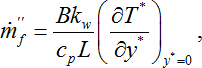
Figure 2 (a) shows these non-dimensional temperature gradients along the length of the fuel surface. They are clearly highest at the leading edge of the fuel surface, where the flame is closest to the fuel surface, and decrease toward the trailing edge (x = 100 mm), where the flame is farthest from the fuel surface. The non-dimensional temperature gradients can be used to determine the local mass-burning rate by applying the correlation^4,6,

     (8)

where B is the mass transfer number of the given fuel, k_w the thermal conductivity of air evaluated at the wall temperature, c_p the specific heat of the air evaluated at an adiabatic flame temperature of the fuel, and L the length of the pyrolyzing fuel surface. The local mass burning rate is then found to vary in a manner similar to the non-dimensional temperature gradients, shown in Figure 2 (b).

Unlike liquid fuels, for PMMA the local mass-burning rate can also be approximated a posteriori by measuring local surface regression over fixed intervals of time^2,11. PMMA samples were burned under representative conditions for periods of time starting at 50 sec and increasing at 50 sec intervals followed by extinction of the sample. The pyrolysis mass flow rate for PMMA is computed at each x location along the central symmetry axis using a first-order approximation given by Pizzo et al.¹¹, discussed in the literature elsewhere^4-6. An average density of PMMA, ρ_s = 1,190 kg/m³ was used along with measured surface regression along the fuel surface to arrive at mass-loss rates during each 50 sec interval along the length of the fuel sample. Although a shorter time step would be desirable, errors in measurement make it become impractical when time steps are less than 50 sec⁵.

To compare local mass-loss rates from thermocouples with those from regression profiles, data from fuel burnout times of 100 and 150 sec were used to compare the local mass burning rates shown in Figure 2 (b). These times correspond to approximately the same times these measurements were taken. As can be seen in the figure, both methods of measuring the local mass burning rate appear very close to one another, suggesting the methodology works well for these types of flames.

For convectively-dominated flames such as these small, laminar ones, temperature gradients at the fuel surface can also be used to extract convective heat fluxes as they are, in essence, directly related to the temperature gradient at the surface. Using measured mass-loss rates, components of flame heat flux can also be extracted along the pyrolysis zone. Using several approximations to the heat balance at the fuel surface, listed in literature elsewhere^2-3, these components can be determined over the surface of a burning slab of PMMA. Figure 3 shows this result, for a PMMA flame stabilized with an ambient free-stream velocity of U_∞= 2.06 m/sec. The technique can therefore be extremely useful in evaluating several measures to describe the burning of small samples of fuels, leading to increased understanding of the combustion process, particularly the relationship between the solid and gas phase.

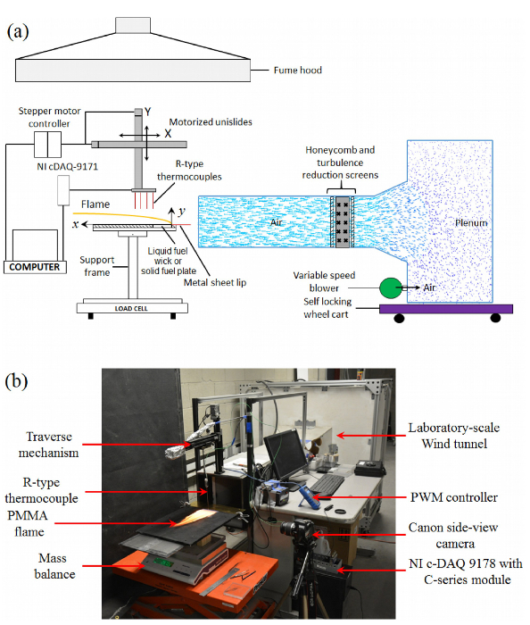
Figure 1. Experimental Setup. (a) Schematic of the experimental setup used to measure mass-loss rates and temperature profiles over a forced-convection boundary layer diffusion flame. (b) Experimental setup for investigating boundary layer diffusion flames under forced flow. Please click here to view a larger version of this figure.

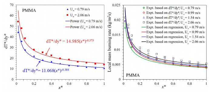
Figure 2. Temperature Gradient and Local Burning Rate Results. (a) Variation of the normal non-dimensional temperature gradients along the fuel surface for a PMMA boundary layer diffusion flame at U_∞= 0.79 m/sec and 2.06 m/sec, respectively. (b) Variation of the local mass-burning rates for PMMA boundary layer diffusion flames at different free-stream conditions. Local mass burning rates obtained through non-dimensional temperature gradients is compared against the experimental data obtained through regression of the PMMA surface. Please click here to view a larger version of this figure.

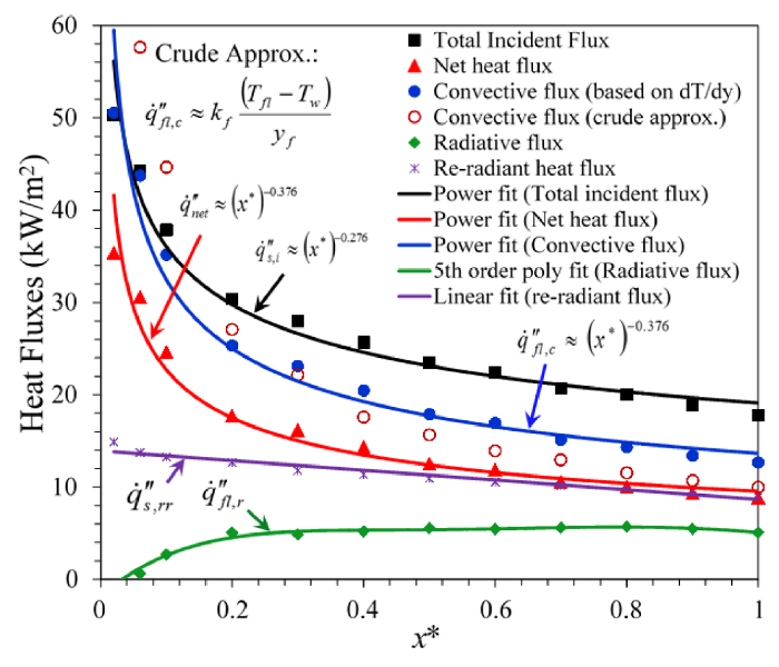
Figure 3. Heat Flux Results under Forced Flow. Distribution of various components of flame heat flux in the pyrolysis zone for a PMMA boundary layer diffusion flame at U_∞= 2.06 m/sec. Please click here to view a larger version of this figure.

Discussion

The goal of this investigation was to develop a new methodology for the estimation of local mass burning rates for both liquid and solid fuels under a variety of flow-field conditions. The study considered two cases, a free convection boundary layer diffusion flame and forced convection boundary layer diffusion flames established under different free-stream conditions, using both liquid and solid fuels.

Local burning rates measured via fine-wire thermocouple measurements over both liquid fuel-soaked wicks and over solid slabs of PMMA were found to match other means of estimation, namely fuel regression measurements. These temperature gradients near the fuel surface were determined using a correlation based upon the Reynolds analogy^12-13 that, while requiring steady, laminar combustion, worked very well for small scale samples, ultimately resulting in data within 15% accuracy for mean results and much more for local measurements^4-6. The correlating factor for these local mass-loss rate measurements depends upon the Spalding mass transfer number of the representative fuel and other thermo-physical properties of the fuel which can be calculated a priori. The results suggest that this technique may be useful to extract these quantities and understand the burning of small scale fuels in greater detail in the future.

Other studies in the literature have expanded the representative work here incorporating numerical simulations⁴ and experiments on vertically-oriented samples, freely burning^4,5, and horizontally-mounted samples under ambient winds⁶. For these configurations, components of heat fluxes have also been determined locally over the fuel surface using the same fine-wire thermocouple technique very close to the condensed fuel surface. While components of heat flux have been measured in the past by use of embedded gauges, this technique is minimally invasive and offers direct measurement of convective heat fluxes, which has not been possible before.

Particular care should be taken during experiments when choosing specific configurations and setup of the apparatus. In these experiments, thermocouples chosen for step 3.2 protruded from a small ceramic tube, keeping tension on the wire and making the location of the thermocouple relatively fixed. Using a thermocouple wire suspended over the entire flame without a tube would reduce possible disturbances from the ceramic tube, however it would make locating the specific location of the thermocouple much more variable as the wire tends to expand with increasing temperatures. Sometimes changes in the configuration could induce effects across the width of the sample (for instance inclining the sample). If the setup is modified from those studied in the past^4-6, around step 4.14 occasional checks that the flame temperature measurements across the width of the sample show no significant variation should be taken (i.e., a 2-D assumption still holds). Otherwise, a 3-D mapping system will need to be implemented.

The most critical steps while performing the experiments have to do with preparation of the fuel and proper use of thermocouples. Even slight deviations in positioning of the thermocouples could cause errors, therefore care must be taken when positioning the thermocouple in steps 3.2, 4.13 and 4.14. The fuel wick must also be placed so that as flat a surface as possible is maintained (step 2.1) and all filler material should be baked out of wicks (step 2.1.1).

The exhaust system, activated in step 4.1 should also be kept as minimal or isolated as possible close to the experiment to help eliminate flow disturbances. This should be checked by ensuring a small candle is not blown where the test will take place (without wind). Baffles, screens, a separate enclosed facility or testing in a large space can be used to accomplish this. In step 4.2, the solid fuel must be ignited as uniformly as possible. While the propane torch is not the most ideal source to do this, experiments were not found to be sensitive to the ignition source in past work^4-6. Sensitivity to the ignition source should be documented during experiments by varying the time or intensity of exposure and observing the results on the steady mass burning rate. If sensitivity is observed a radiant panel should alternatively be used to ignite samples. Solid fuels, or any fuel that does not have a large (>300 sec) steady burning region as observed by mass-loss rates should have temperature mapping taken during a short region. For instance, in step 4.13 the mapping is recommended for PMMA to be taken over the first 150 sec, while the fuel is still relatively flat and surface regression has been well documented. Surface regression measurements can use ImageJ or other similar image software to measure pixels on the photographs and convert to length. Alternatively, a digital micrometer can be used to measure the surface regression of the solid plate after it cools (note the surface of "bubbling" materials such as PMMA must be sanded first).

The proposed burning rate correlation is based upon laminar assumptions, however, it is hypothesized that this technique should follow a similar form for turbulent burning of a fuel surface, albeit with a modified functional relationship which must be experimentally determined. The work presented here can be subsequently extended to turbulent boundary layer combustion and associated interactions between turbulence and gas-phase heat release that drive the incident heat flux to the fuel surface can be further investigated.

The theory upon which the burning rate correlation is based also neglects radiation. The theory is oversimplified leading to uncertainty in its predictive capabilities in circumstances that are not covered by the present work. For instance, the given methodology may not work for high sooting flames where the heat flux to the surface is largely radiative. For large turbulent wall flames, where radiative heat flux to the condensed fuel surface is high, the proposed burning rate correlation may or may not work. Inclusion of radiation effects in the proposed correlation is, thus, desirable and further research must be undertaken in order to determine this functional relationship. This area requires improvements in the model if confident prediction methods are to be achieved for such flames.

Materials

List of materials used in this article

Name	Company	Catalog Number	Comments
Thermocouples with connectors and clamps
Unsheathed Fine Gauge T/C	P13R-002	Omega Engineering, Inc.	Fine wire microthermocouples (R-type)
Unsheathed Fine Gauge T/C	P13R-003	Omega Engineering, Inc.	Fine wire microthermocouples (R-type)
Ceramic 2 hole round - 5 pk	TRX-010364-6	Omega Engineering, Inc.	Ceramic tubes to hold the fine wire thermocouples
Thermocouple extension wire	EXTT-RS-24-100	Omega Engineering, Inc.	Thermocouple extension wire
Male Female Connectors	SHX-R/S-MF	Omega Engineering, Inc.	Connectors for R-type thermocouples
Accessories	MSRT-116-10	Omega Engineering, Inc.	Rubber tubes for maintaining grip for the ceramic tubes at the connectors's end
Traverse mechanism
X slide, travel = 10 inch, 0.025 in/rev, limits, NEMA 17	XN10-0100-E25-71	Velmex Inc.	Velmex unislide
Vexta type 17, 1.8 deg/step 2phase, single shaft stepper motor	PK245-01AA	Velmex Inc.	Stepper motor
Mounting cleat, standard using 6-32 bolts	XMC-2	Velmex Inc.	Mounting accessories for the given Velmex unislide
6-32 x 7/16 SH Cap Screw for Xslide in X & Y axis	XMB-1	Velmex Inc.	Mounting accessories for the given Velmex unislide
X slide, travel = 10 inch, 0.025 in/rev, limits, NEMA 17	XN10-0100-E25-71	Velmex Inc.	Velmex unislide
Vexta type 17, 1.8 deg/step 2phase, single shaft stepper motor	PK245-01AA	Velmex Inc.	Stepper motor
Mounting cleat, standard using 6-32 bolts	XMC-2	Velmex Inc.	Mounting accessories for the given Velmex unislide
6-32 x 7/16 SH Cap Screw for Xslide in X & Y axis	XMB-1	Velmex Inc.	Mounting accessories for the given Velmex unislide
Control, 2 Axis programmable stepping motor control, 1 motor at a time	VXM-2	Velmex Inc.	Stepper motor controller
USB to RS232 DB9 Serial Communication cable 10 ft	RPC-USB-RS232-3M	Velmex Inc.	Serial communication cable between the stepper motor controller and  computer
Data acquisition hardware
NI 9214 16-Ch Isothermal TC, 24-bit C Series Module for high accuracy thermocouple measurements (includes terminal block)	781510-01	National Instruments	Thermocouple data acquistion card
Power Cord, AC, U.S., 120 VAC, 2.3 meters	763000-01	National Instruments	Power cord for the 8 slot C-DAQ chassis
cDAQ-9178, CompactDAQ chassis (8 slot USB)	781156-01	National Instruments	C-DAQ chassis for NI 9214 and NI 9239
EMI Suppression Ferrite for NI 9229/39 BNC	782801-01	National Instruments	Accessories for NI 9239 data acquistion card
NI 9239 BNC, 4-Ch +/-10 V, 50 kS⁠/⁠s per channel	780181-01	National Instruments	Data acquistion card for hot wire anemometer system
cDAQ-9171, CompactDAQ chassis (1 slot USB)	781425-01	National Instruments	C-DAQ chassis for NI 9214
Cameras
Nikon D7100 24.1 MP DX-Format CMOS Digital SLR with 18-105 mm f/3.5-5.6 AF-S DX VR ED Nikkor Lens	Nikon D7100	Amazon	Digital SLR camera for taking top-view flame photographs
Canon EOS Rebel T5 DSLR CMOS Digital SLR Camera and DIGIC Imaging with EF-S 18-55 mm f/3.5-5.6 IS Lens	Canon EOS Rebel T5 DSLR	Amazon	Digital SLR camera for taking side-view flame photographs
Mass balance
Mettler-Toledo, MS32001L Balance Prec 32,200 g x 0.1 g	97035-654	VWR	Precision electronic mass balance for measuring average mass burning rate
Mini CTA system
MiniCTA Anemometer Package for wire- and film-probes	9054T0461	Dantec Dynamics	Hot wire system for measuring velocities and turbulence intesity at the wind tunnel outlet
Wind tunnel equipment
1/2 in. x 4 ft. x 8 ft. C-3 Whole Piece Birch Domestic Plywood	Model # 833185	Home Depot	Used to make the laboratory scale wind tunnel
Woodgrain Millwork WM 206 11/16 in. x 11/16 in. x 96 in. Wood Pine Corner Moulding	Model # 109610	Home Depot	Used to make the laboratory scale wind tunnel
Extension Spring, Loop Ends, 6.562" Overall Length, Pack of 6	1330K26	McMaster-Carr	Used to make the laboratory scale wind tunnel
Strainer Grade Wire Cloth, 30x30 Mesh, 0.0130" wire diameter. 12"x12" sheet	9241T41	McMaster-Carr	Used to make the laboratory scale wind tunnel
Strainer Grade Wire Cloth, 40x40 Mesh, 0.0065" wire diameter. 12"x12" sheet	9241T42	McMaster-Carr	Used to make the laboratory scale wind tunnel
Mobile Lift Table Foot-Operated, 600# Capacity, 10" - 33" Table Height	2791T22	McMaster-Carr	Table to hold the experimental setup
ebm-papst p/n: G3G250-MW75-05 (EC Centrifugal blower, 200-240 V, 3-phase, 50/60 Hz, M3G112-EA motor, 2.2 kW)	G3G250-MW75-05	Ebm papst	Blower for the wind tunnel
ebm-papst p/n: HX0C-003-000-04 (Controller)	HX0C-003-000-04	Ebm papst	Pulse width modulation controller for controlling the speed of the blower
8020 1” X 1” T-SLOTTED PROFILE	8020-1010	80/20 (Rankin Automation)	Used to create a framework for the wind tunnel
Momentive/GE Silicone Sealant RTV108, 10.1-oz Cartridge, Semi-Clear	7545A472	McMaster Carr	Sealant for the wood
Software
LabVIEW	Contact vendor	National Instruments	Used for continuous temperature data acquistion and analysis. Alternatively used for positioning the thermocouple.
Mettler Toledo mass balance software	Contact vendor	Mettler Toledo	Used for measuring the mass loss rate of the condensed fuel wick / solid plate with time
ImageJ	Free download	NIH, http://imagej.nih.gov/ij/	Used for measuring the flame standoff distance and surface regression of the solid fuel plate
Matlab	Contact vendor	Mathworks	Used for post-processing of data
Fortran 90/95	Contact vendor	The Fortran company	Used for post-processing of data
Materials
Methanol	UMD Chem Store	NA	Liquid fuel
Ethanol	UMD Chem Store	NA	Liquid fuel
safety glasses	UMD Chem Store	NA	Used for safety purpose
spray bottle	UMD Chem Store	NA	Used for carrying water in case of emergency
Syringe 60 cc	UMD Chem Store	NA	Used for soaking the liquid fuel wick with liquid fuels
Optically Clear Cast Acrylic Sheet, 1/8" Thick, 24" x 48"	Mc master carr	8560K262	Solid fuel PMMA
Loctite Proxy Pak (Hi-temp adhesive)	Mc master carr	7556A33	Used for covering the sides of the wick with aluminum foil
Hi-Temp Aerosol Spray Paint (Black)	Mc master carr	7832T1	Used for painting the insulation
Self-Igniting Economy Propane Gas Torch Adjustable Flame, 4,179 Btu/hr	Mc master carr	78245A3	Propane torch for igniting the solid fuel plate
Heat-Resistant Cotton Glove W/Nitrile Coating, 400 Deg F Max Temp, 10" Lg, Large	Mc master carr	56025T1	Used for safety purpose
Modular Protective Screen with Tie-on Curtain, 6' Height x 4' Width Abrasion-Resistant Fiberglass	Mc master carr	9145T84	Fire-resistant curtain for the background
Multipurpose Aluminium Alloy 6061 .125" thick, 12" x 24"	Mc master carr	89015K28	Used for holding the insulation
Marine grade plywood 1/2" thick, 12" x 24"	Mc master carr	1125T32	Used for holding the experimental setup
Multipurpose Aluminium Alloy 6061 U-channel, 2" base x 1-1/4" legs, 1' length	Mc master carr	1630T473	Used for holding the aluminum plate, insulation and wick
Architectural Anodized Aluminium (Alloy 6063) 90 deg angle, 1/8" Thk, 1/2" x 1/2" legs, 6' L	Mc master carr	4630T21	Used for holding the aluminum plate, insulation and wick
Aluminium Inch T-Slotted Framing System Concealed 90 degree connector, for 1" extrusion	Mc master carr	47065T155	Used for holding the aluminum plate, insulation and wick
Aluminium Inch T-Slotted Framing System Extended 90 degree bracket, Single, 4 Hole, for 1" extrusion	Mc master carr	47065T175	Used for holding the aluminum plate, insulation and wick
Aluminium Inch T-Slotted Framing System Four-Slot single, 1" solid extrusion, 4' length	Mc master carr	47065T101	Used for holding the aluminum plate, insulation and wick
1/2" x 48" x 36" (Superwool 607 insulation board) 1 carton containing 12 sheets	Mccormick Insulation	Superwool 607	Insulation material for making the wick and the wick holder

References

- Babrauskas, V., Peacock, R. D. Heat release rate: the single most important variable in fire hazard. Fire Safety J. 18 (3), 255-272 (1992).
- Pagni, P., Shih, T. M. Excess pyrolyzate. Proc. Combust. Inst. 16 (1), 1329-1343 (1977).
- Orloff, L., Modak, A. T., Alpert, R. Burning of large-scale vertical surfaces. Proc. Combust. Inst. 16 (1), 1345-1354 (1977).
- Singh, A. V., Gollner, M. J. Estimation of local mass burning rates for steady laminar boundary layer diffusion flames. Proc. Combust. Inst. 35 (3), 2527-2534 (2015).
- Singh, A. V., Gollner, M. J. A methodology for estimation of local heat fluxes in steady laminar boundary layer diffusion flames. Combust. Flame. 162 (5), 2214-2230 (2015).
- Singh, A. V., Gollner, M. J. Local burning rates and heat flux for forced flow boundary-layer diffusion flames. AIAA J. 54 (2), 408-418 (2016).
- Collis, D., Williams, M. Two-dimensional convection from heated wires at low Reynolds numbers. J. Fluid Mech. 6 (3), 357-384 (1959).
- Jakob, L. M. Heat Transfer. , Wiley. New York, USA. (1967).
- Sforza, P., Steiger, M., Trentacoste, N. Studies on three-dimensional viscous jets. AIAA J. 4 (5), 800-806 (1966).
- Pizzo, Y. Experimental observations on the steady-state burning rate of a vertically oriented PMMA slab. Combust. Flame. 152 (3), 451-460 (2008).
- Chilton, T. H., Colburn, A. P. Mass transfer (absorption) coefficients prediction from data on heat transfer and fluid friction. Ind. Eng. Chem. 26 (1), 1183-1187 (1934).
- Silver, R. Application of the Reynolds analogy to combustion of solid fuels. Nature. 165, 725-726 (1950).
Reprints and Permissions