Fiber Optic Distributed Sensors for High-resolution Temperature Field Mapping

Summary

We demonstrate use of a fiber optic distributed sensor for mapping the temperature field of mixing air jets. The Rayleigh scattering-based sensor generates thousands of data points along a single fiber to provide exceptional spatial resolution that is unattainable with traditional sensors such as thermocouples.

Abstract

The reliability of computational fluid dynamics (CFD) codes is checked by comparing simulations with experimental data. A typical data set consists chiefly of velocity and temperature readings, both ideally having high spatial and temporal resolution to facilitate rigorous code validation. While high resolution velocity data is readily obtained through optical measurement techniques such as particle image velocimetry, it has proven difficult to obtain temperature data with similar resolution. Traditional sensors such as thermocouples cannot fill this role, but the recent development of distributed sensing based on Rayleigh scattering and swept-wave interferometry offers resolution suitable for CFD code validation work. Thousands of temperature measurements can be generated along a single thin optical fiber at hundreds of Hertz. Sensors function over large temperature ranges and within opaque fluids where optical techniques are unsuitable. But this type of sensor is sensitive to strain and humidity as well as temperature and so accuracy is affected by handling, vibration, and shifts in relative humidity. Such behavior is quite unlike traditional sensors and so unconventional installation and operating procedures are necessary to ensure accurate measurements. This paper demonstrates implementation of a Rayleigh scattering-type distributed temperature sensor in a thermal mixing experiment involving two air jets at 25 and 45 °C. We present criteria to guide selection of optical fiber for the sensor and describe installation setup for a jet mixing experiment. We illustrate sensor baselining, which links readings to an absolute temperature standard, and discuss practical issues such as errors due to flow-induced vibration. This material can aid those interested in temperature measurements having high data density and bandwidth for fluid dynamics experiments and similar applications. We highlight pitfalls specific to these sensors for consideration in experiment design and operation.

Introduction

Computational fluid dynamics (CFD) codes are used to simulate a wide variety of fluid systems, from airflow around planes and automobiles down to arterial blood flow. The scope and fidelity of such simulations have grown with the availability of computing power. However, despite the sophistication of advanced simulations, their accuracy and reliability are often hard to quantify. In practice, the accuracy of CFD codes is assessed by comparing simulations with experimental data in a process called code validation.

A typical experimental data set consists chiefly of velocity and temperature measurements, both ideally of high spatial and temporal resolution to facilitate rigorous code validation. Velocity fields can be mapped at high resolution using particle image velocimetry (PIV), a well-established optical technique^1,2. In contrast, it is difficult to map temperature fields with resolution comparable to that of PIV. Optical techniques such as laser-induced fluorescence are available^3,4, but they require cameras and relatively high-power lasers, and are unsuitable for opaque fluids.

An alternative is available in the relatively new technique of distributed temperature sensing based on Rayleigh scattering and swept-wavelength interferometry (SWI)^5-7. Thousands of temperature measurements can be acquired along a single optical fiber. A distributed temperature sensor (DTS) can span large flow fields and function in environments that are unsuitable for image-based techniques⁸. There are also DTSs based on Raman and Brillouin scattering^9,10, but sensors based on Rayleigh scattering and SWI provide spatial and temporal resolution more suitable for typical fluid dynamics experiments.

Though DTSs offer data density far beyond that of traditional sensors such as thermocouples (TCs), sensors based on Rayleigh scattering respond to strain as well as temperature¹¹. If the fiber coating is hygroscopic, sensors also respond to humidity changes^12,13. Absorption of water vapor swells the coating while desorption shrinks it¹⁴, which strains the underlying glass fiber and alters the signal. As a result, accuracy is affected by handling, vibration, and shifts in relative humidity. This is quite unlike traditional sensors and so unconventional installation and measurement methods must be observed to obtain accurate data. This paper demonstrates the use of a DTS in a thermal mixing experiment, presenting a protocol and guidelines to ensure accuracy.

The DTS used here is based on detection and analysis of Rayleigh scattering within a fiber optic waveguide. A random distribution of impurities and structural variations along the fiber core gives rise to a backscatter pattern that is unique to the fiber and generally stable. The spectrum and amplitude of this pattern can be read to serve as a fiber signature. Physical changes such as temperature shifts or strain alter the signature in a repeatable way, and detecting signature variations is the basis for using the fiber as a sensor.

Figure 1 illustrates the principle components of the optoelectronic sensing device, called an optical distributed sensor interrogator, and denoted here simply as "interrogator". In a technique known as swept-wavelength interferometry, a low power tunable laser launches a narrow band signal into the fiber for the purpose of registering resultant backscatter^5-7. The laser is swept across an interval of several nanometers and the signal split between reference and measurement legs. Scattered light from the sensor is combined with the reference signal to generate interference signals at the detectors. Detector output is digitized and analyzed to retrieve the Rayleigh scattering signal. The Rayleigh signature of the sensor shifts in wavelength where sensor temperature (strain, or humidity) changes. The magnitude of this wavelength shift is related to sensor sensitivity, which is a physical constant associated with the fiber type, which has a calibration factor analogous to the Seebeck coefficient of a TC.

Figure 2 shows the glass tank that serves as the test section used in this study. The camera behind the tank gives a sense of scale. Air enters through two hexagonal ducts and mixes before exiting through a vent. To highlight the jets, one flow stream was seeded with oil mist while the other remained pure air. The tank lid has a window covered with a black polymer screen. Though not visible in the photo, the DTS is suspended below the black screen.

A 50 m long DTS was mounted below the tank lid as shown in Fig. 3. It was fashioned from 155 µm diameter polyimide-coated optical fiber and hung on 127 µm diameter steel wire strung between tank end panels. The sensor was woven through the wire in an alternating pattern and looped back and forth across the tank 49 times. It spans a 0.5 x 0.8 m plane and generates 1,355 independent data points at 4 Hz and spatial resolution of 30 mm, 4,067 data points when oversampled with 10 mm spacing. Such high density temperature data complements velocity data and increases the value of data sets for CFD validation. The protocol outlines the process of sensor selection, fabrication, and configuration while focusing on the particular concerns in using the DTS in a fluid dynamics experiment.

Protocol

1. Select Optimal Sensor Type for Application

1. Choose sensor length based on tradeoff between sampling speed and number of data points.
   NOTE: One interrogator samples sensors up to 50 m in length at 2.5 Hz and resolution <10 mm while the other samples sensors up to 10 m in length at 5 mm resolution and 100 Hz.
2. Select a type of single mode optical fiber based on requirements for service temperature limits, time response, humidity sensitivity, and installation configuration (bare or in capillary).
   NOTE: Here we have used 155 µm diameter polyimide-coated single-mode commercial telecom optical fiber.
   NOTE: See Tables 1 and 2 as examples of fibers and configurations we have used in our laboratory.

2. Install Optical Fiber in Test Section

1. Open test section by removing one of the long glass side plates.
2. Drill 1 mm diameter holes in side walls 3 mm below lid for wire anchors (Fig. 3).
   NOTE: Anchors hold steel wire that support the sensor. The anchor pitch can be varied in accordance with test section size and expected dynamic loading from flow. The 20 mm pitch used here proved stable with minimal vibration in flow near 1 m/sec. Vibration corrupts DTS signals and is more problematic with long sensors^15,16.
3. String a 127 µm diameter steel wire segment across the test section by tying it to a brass anchor at each end of the tank. Repeat until there are a total of 47 wire segments strung across the tank.
4. Cut 50 m of optical fiber using communications/electricians scissors with reserve to be consumed in splicing connector and termination fiber (likely <0.5 m, but dependent upon proficiency at splicing). Collect this fiber on a small spool, ~50 mm in diameter.
5. Lay the first sensor segment at one edge of the area chosen to measure temperature with the sensor array.
   NOTE: After the first segment is fixed in position, the fiber will be looped for an adjacent segment, fixed in position, and more fiber dispensed for the next segment in a repetitive process that builds the array until all the fiber is used.
6. Weave the fiber above and below adjacent wires, working from one side of the tank to the other, dispensing fiber from the spool as needed.
   NOTE: The fiber is perpendicular to the wire as shown in Fig. 3 with the weave supporting it against the force of gravity in one direction and flow in the other.
7. Attach each end of the first fiber segment to the lid with conventional clear tape or polyimide film tape. The first segment of the array is now in place.
   NOTE: Do not fix sensor taut like a guitar string, but rather taut enough to be straight and take up visible slack. If the sensor is tensioned, small deformations in the support, e.g., thermal expansion of the lid, will change this tension and generate anomalous signal offsets and measurement errors.
8. Loop the fiber 180 degrees to return it back for the next segment as shown in Fig. 4 and tape it to the lid at a distance of 10 mm from the first segment.
   NOTE: Minimize the loop diameter since it is "wasted fiber" (not part of the array), but it should be roughly 30 mm or more for tolerable stresses. The fiber used here has tolerated 30 mm diameter loops for several months with no noticeable signal loss, but limits will vary with fiber type. For the fiber used here, the manufacturer specifies the "short-term" bend radius limit as ≥ 10 mm and "long-term" limit as ≥ 17 mm.
9. Again weave the fiber between wires towards the opposite side of the tank and tape in position. Repeat the looping, taping, and weaving process until all the fiber is used.

3. Splice Connector and Termination to Fiber

1. Splice an LC-type single mode connector to one end of the fiber using a fusion splicer following manufacturer instructions¹⁷.
2. Cut ~0.25 m termination fiber with the electrician/communication scissors and splice to the other end of the fiber, again with a fusion splicer following manufacturer instructions.
   NOTE: This assembly (fiber, connector, and termination) will now be referred to as a "sensor". The termination fiber disperses residual signal from the laser pulse to prevent it from returning to the interrogator.

4. Sensor Configuration

1. Plug the LC-type connector end of the sensor into the interrogator port and start configuration software.
2. Generate sensor amplitude data by selecting "acquire" (distinct from temperature data), which is automatically displayed when the scan is complete.
   NOTE: The trace for a sensor with good splices will have the general characteristics shown in Fig. 5. A poor splice may be indicated by an indistinct noise floor or dominant reflection where the connector is expected. If a poor splice is suspected, return to step 3 and repeat splicing procedure.
3. Select the active portion of the sensor by dragging the yellow cursor shown on the screen to the beginning of the sensor and the red cursor to the end.
4. Give the sensor a name and select "save sensor files".
   NOTE: The sensor is now configured and ready for use.
5. Close the configuration software and switch to the measurement software.

5. Map Sensor Position within Test Section

1. Start the interrogator measurement software and load the sensor just configured.
2. Connect a soldering iron to a variable transformer set to ~40%, preheating for 5-10 min.
   NOTE: The soldering iron generates local temperature spikes for mapping. A soldering iron can melt the fiber coating and ruin the sensor so start with a low transformer setting, using just enough power to obtain clear spikes. A 10-20 °C spike suffices for this process.
3. Select "measure" in the interrogator software to plot live data on screen.
4. Zoom out to display the entire sensor on the screen.
5. Hold soldering iron near sensor and briefly touch it at the first mapping point, here the segment furthest from the vent where it meets the lid (Fig. 4).
6. Record position of temperature peak as indicated by software along with the corresponding physical location within test section.
7. Repeat 5.5-5.6 to map the end points of all 49 segments.

6. Sensor Baseline: The Link to Absolute Temperature

1. Position one or more temperature standards, e.g., TC or resistance temperature detector (RTD), near the DTS to serve as the standard linking DTS readings to absolute temperature.
2. Close up the tank by replacing the long glass side plate that was removed in step 2.1.
3. Insulate the tank by wrapping it in blankets or conventional insulation panels and allow it to sit overnight to establish an isothermal atmosphere.
4. Start the interrogator software, select "baseline" (or "tare"), and simultaneously note/record the TC (or RTD) reading. When software is finished with the baseline, select "measure" to plot live data to examine the quality of the baseline.
   NOTE: This critical step establishes the DTS baseline and the signal should now indicate zero, i.e., ΔT(x)=0 ± a fraction of a degree. From now on, the signal will vary as tank temperature diverges from the reference temperature: ΔT(x) = T(x)_abs - T_base, where T(x)_abs is the absolute temperature along the fiber and T_base is the baseline temperature^6,18. If the test section is nonisothermal, T_base will be a function of position, i.e., T_base(x), and accuracy will be compromised unless T_base(x) is mapped with more than one TC or RTD (see discussion section). Do not move or touch the sensor until step 7 is completed. Straining it in any way can introduce offsets that may degrade measurement accuracy.
5. Examine the live signal, which should not drift far from zero. If drift is excessive for application (our limit is roughly 0.5 °C after ~5 min), allow more time for test section to reach thermal equilibrium and/or improve insulation (see note below) and then repeat step 6.4.
   NOTE: Signal quality is always best immediately after baseline and will drift over time depending on the temperature distribution within the test section. Good insulation and long waiting periods before base lining will reduce drift and measurement error. Sizeable, rapid drifts indicate the test section is not isothermal, which will ultimately lead to inaccurate measurements.
6. Select the logging function in the interrogator software and record 10-100 scans of DTS data for the same stagnant, isothermal conditions just used to generate the baseline. Record also the TC/RTD reading.
   NOTE: This is reserve data for posttest checks of offsets that may be generated by strain from flow or unexpected deformation of the test section or supports.

7. Run Test

1. Turn on the compressor to generate air flow and adjust flow controllers to match flow rates at 1.25 kg/sec to each channel.
   NOTE: Average inlet velocity is 1.1 m/sec and Reynolds number is 10,000.
2. Set heater power to 600 W to warm the east jet 20 °C above the west jet, which is at ambient temperature.
3. Allow the system to run overnight to reach equilibrium.
4. The next day examine live DTS signal to assess noise levels. Select the sensor "gage length" in the software to achieve acceptable noise levels (a 30 mm gage is used here).
   NOTE: Gage length corresponds to sensor spatial resolution. In general, signal noise increases as gage length decreases and as flow-induced vibration increases (see user guide and reference 13 and 14).
5. Log 2,000 DTS scans at 4 Hz.
6. Turn off heater power and air flow. Let the tank sit overnight to reach equilibrium and record 10-100 DTS scans to complement the pre-test data set saved for posttest offset checks.

8. Data Analysis

1. Select the post processing feature in the main window of the interrogator software and import the test data, which is in a proprietary binary format.
2. Export the data as a plain text file that can be read by conventional spreadsheet programs.
   NOTE: This data represents measured ΔT along the fiber where ΔT(x) = T(x)_abs - T_base. It contains no reference to position in the test section (see Fig. 6). Additional details are available in the interrogator user's guide and references 6 and 16 for this step and the next.
3. Import text data into a conventional spreadsheet and convert to absolute temperature by adding T_baseline, measured by TC or RTD in step 6.4, to all data.
   NOTE: The conversion to absolute temperature is simply a single-value offset correction: T(x)_abs = ΔT(x) + T_baseline since we have stipulated that the test section was isothermal during baseline.
4. Use spreadsheet software or similar data manipulation program to decompose T(x) data and map it to physical positions within the test section like that shown in Figures 7 and 8.
   NOTE: The program will utilize the data collected with the soldering iron in step 5.

Results

Raw DTS data is plotted in Fig. 6 showing measured ΔT from the baseline temperature (roughly 20 °C) versus distance along the sensor. The data is "raw" in the sense that it has neither been converted to absolute temperature nor mapped to physical positions within the test section. Data is based on a 30 mm gage length, which provides 1,666 independent measurements over the full sensor length of 50 m. The 30 mm gage was applied at 10 mm intervals in an oversampling mode that increases the number of data points to 5,000. Such data density is not practicable with conventional sensors such as TCs.

At x=0 in Fig. 6 the sensor is at the east end of the tank, and as x increases it loops back and forth towards the west end. Peaks occur where the sensor passes over the hot east jet and then fade where it is over the cold west jet. The plot illustrates how even the raw signal from a single DTS can provide a basic portrayal of temperature over a rather wide region. Note the signal noise towards the west end of the fiber, which is due to flow-induced vibration. Though vibration was not visible to the naked eye, it was sufficient to degrade the signal and we see this problem most often with long sensors (> 10 m).

The raw data is mapped onto the test section in Fig. 7, which shows temperature across the 0.5 x 0.8 m measurement plane formed by the DTS array. The point of view is from above the tank looking down onto the lid. Outlines of the hexagonal channels are included as an orientation aid. The contour is based on 4,067 data points since the loops taped under the lid are excluded. Linear interpolation between adjacent sensor segments was used to create the 2D contour.

The contour provides a clear sense of the thermal pattern beneath the lid with a warm region over the east jet, but not centered around it. Also evident is a rough symmetry around the tank midplane, which is y=0 on the plot. This sort of temperature data is a useful compliment to velocity data in fluid dynamics studies involving thermal mixing and heat transfer. Rigorous code validation requires such high resolution data for both the temperature and velocity fields.

The same sensor data can be processed to reveal the magnitude of temperature fluctuations. The RMS (root mean square) of the 2,000 scan data set is plotted in Figure 8. Magenta marks the region where temperature fluctuations are relatively high. This is also a region of high turbulence where the two rising jets interact as impinge on the lid. RMS data is useful for turbulence modeling in the context of thermal mixing.

Figure 1. Interrogator schematic. Principle components of optical distributed sensor interrogator for temperature measurements. The system is based on swept-wavelength interferometry, which characterizes the sensor's Rayleigh backscatter signature. Please click here to view a larger version of this figure.

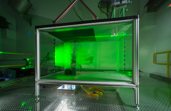
Figure 2. Test section. Air jet mixing experiment: air enters tank through base via two hexagonal ducts and mixes before exiting through top vent. The black screen covering the lid window is 3 mm above the DTS (not visible). Please click here to view a larger version of this figure.

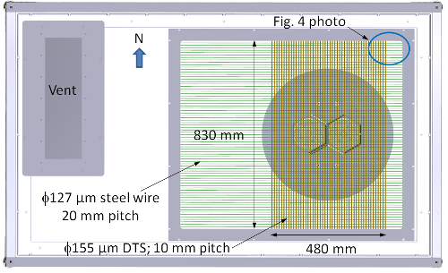
Figure 3. DTS mounting configuration. Top view of tank showing DTS woven between steel support wires strung across the long axis of the tank. Please click here to view a larger version of this figure.

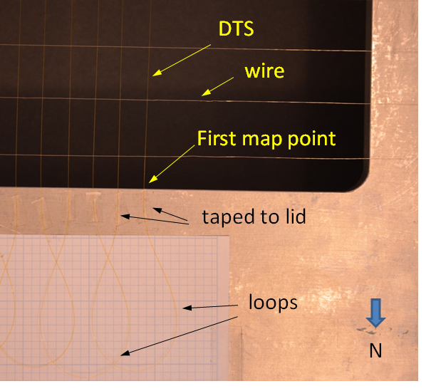
Figure 4. DTS close-up. Close-up photo of DTS with view from inside tank upward at lid to highlight sensor loops, attachment, and location of first test point to be mapped with soldering iron. Please click here to view a larger version of this figure.

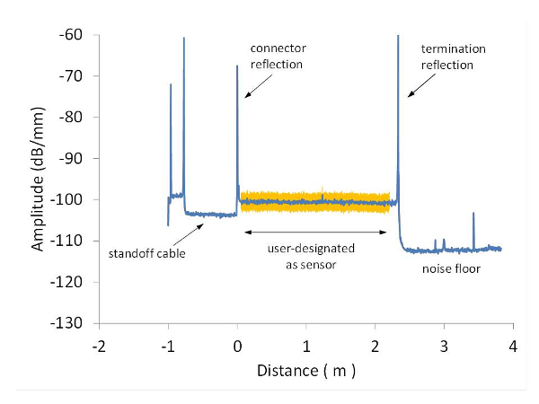
Figure 5. Rayleigh scattering signal. Typical Rayleigh scattering signal recorded with sensor configuration utility (short sensor shown here for clarity). Proper termination will generate sharp signal drop to noise floor. The slight signal step up and modest reflection at the connector is characteristic of a properly spliced connector. Please click here to view a larger version of this figure.

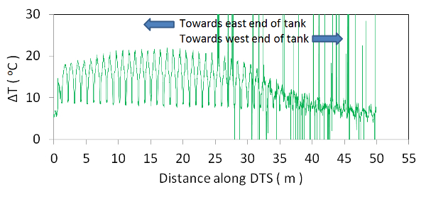
Figure 6. Raw DTS data. A single scan of raw DTS data with the hot east jet at 45 °C and cold west jet at 25 °C. Peaks occur where sensor is directly above hot jet. Recall that the sensor is looping back and forth between tank walls. Please click here to view a larger version of this figure.

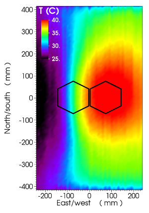
Figure 7. Measured air temperature below lid. DTS raw data converted to absolute temperature and mapped to physical position within tank. Data based on 2,000 scans logged at 4 Hz. Data spacing 10 mm for a total of 4,067 plotted data points. Linear interpolation used to fill regions between sensor segments. Hexagons show positions of inlets. Please click here to view a larger version of this figure.

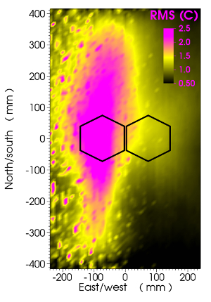
Figure 8. Root mean square (RMS) of measured temperature. RMS of data plotted in Fig. 7. Magenta indicates high temperature fluctuations and thermal mixing of hot and cold jets. Hexagons show positions of inlets. Please click here to view a larger version of this figure.

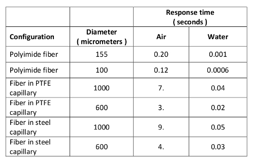
Table 1. Order of magnitude thermal response time for selected fiber types and housing configurations in cross flow at 1 m/sec and 20 °C.

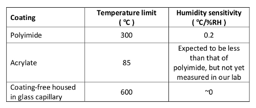
Table 2. Approximate operating temperature limits and humidity sensitivities for selected coating configurations.

Discussion

We have demonstrated the use of a DTS in a fluid dynamics experiment. The main advantage of these sensors is the great number of measurement points that can be obtained from a single sensor. The DTS used here generated data at 4,067 points across a 0.5 x 0.8 m plane, far beyond the practicable limits of conventional point sensors such as thermocouples. While such data density can be exceeded by optical techniques such as laser induced fluorescence (LIF), a DTS will function in opaque fluids and applications that lack optical access. The high data density of a DTS is suitable for experiments involved in computational fluid dynamics code validation.

Baselining is the critical step in the protocol and central in determining measurement accuracy. An isothermal test section is essential to ensure the entire DTS is at one temperature when baselined. If this is not possible, T_base becomes T_base (x), which should be mapped by multiple TCs placed in close proximity to the DTS. Though baseline quality can be improved in this fashion, it complicates the process of mapping the DTS baseline to the standards for conversion to absolute temperature.

Always be on the lookout for sources of strain after the baseline, which can introduce unpredictable signal shifts. Such sources are, for example, test section thermal expansion that stretches the sensor, movement of supports, dynamic loading from high flow rates, or flow-induced vibration. The pre- and posttest measurements under isothermal conditions will help identify such problems.

Strain sensitivity is the main shortcoming of this Rayleigh scattering-based DTS. Unlike conventional sensors like thermocouples, it is sensitive to handling, humidity, and vibration. These issues are most relevant for the bare sensor configuration demonstrated here, but far less important for sensors housed in capillaries.

Unlike conventional sensors, a DTS cannot be procured with paperwork tracing it to a recognized calibration standard such as NIST (National Institute of Standards and Technology). In-situ calibrations are necessary, preferably with an isothermal test section, which may be difficult in some applications. Vibration is of special concern for bare fiber strung across a large test section. We have had mixed success with a vertically-oriented array that spans the long axis of the tank at segment lengths of 1.7 m. A configuration with 28 m of fiber and 16 segments performed well during one study¹⁸, but attempts to extend it to 53 m with 29 segments was unsuccessful¹⁶.

In general, signal noise for any sensor length and configuration can be decreased by increasing the gage length over which the interrogator software calculates the Rayleigh signal shift, but this reduces effective spatial resolution. Each application must strike its own balance between signal noise and spatial resolution. Again, such difficulties can be largely avoided by housing the sensor in a capillary at the expense of extended thermal response time.

This relatively new temperature measurement technology requires development to reduce susceptibility to vibration. Much of this work will necessarily involve the interrogator hardware and software. The sensors themselves may also be improved to reduce sensitivity to handling and humidity changes, which are affected by the fiber coatings. Work could focus on developing coatings superior to the polyimide and acrylate-coated fibers currently commercially available.

Materials

List of materials used in this article

Name	Company	Catalog Number	Comments
Sensor interrogator	Luna Inc.	ODiSI-A and -B	The two systems differ primarily in speed and spatial resolution
Fusion splicer	Fujikura	70S
Cleaver	Fujikura	CT-3A
3-hole jacket stripper	Fiber Instrument Sales	F11301T
Optical fibers	OFS, Specialty Photonics Division	BF06160-02	Polyimide coating
Optical fibers	Newport Corp.	F-SM1500-4.2/50	Acrylate coating
Connector	AFL Global	FUSE-LC-9U-SMA-6
Termination fiber	OFS, Specialty Photonics Division	552 HPWR 040

References

- Raffel, M., Willert, C., Wereley, S., Kompenhans, J. Particle Image Velocimetry. , Springer. New York. (2007).
- Adrian, R. J. Twenty years of particle image velocimetry. Exp. Fluids. 39, 159-169 (2015).
- Vetrano, M. R., Simonini, A., Steelant, J., Rambaud, P. Thermal characterization of a flashing jet by planar laser-induced fluorescence. Exp. Fluids. 54, 1573-1583 (2013).
- Dahikar, S. K., Sathe, M. J., Joshi, J. B. Investigation of flow and temperature patterns in direct condensation using PIV, PLIF and CFD. Chem. Eng. Sci. 65, 4606-4620 (2010).
- Juškaitis, R., Mamedov, A. M., Potapov, V. T., Shatalin, S. V. Distributed interferometric fiber sensor system. Opt Lett. 17 (22), 1623-1625 (1992).
- Gifford, D., et al. Swept-wavelength interferometric interrogation of fiber Rayleigh scatter for distributed sensing. Proc. SPIE. 6770, Fiber Optic Sens and Appl V. 67700F (2007).
- Kreger, S., Gifford, D., Froggatt, M., Soller, B., Wolfe, M. High resolution distributed strain or temperature measurements in single- and multi-mode fiber using swept-wavelength interferometry. Optical Fiber Sensors. 2006, OSA/OFS 2006 4 (2006).
- Bersan, S., et al. Application of a high resolution distributed temperature sensor in a physical model reproducing subsurface water flow. Measurement. , http://dx.doi.org/10.1016/j.measurement.2015.09.018 (2015).
- Bao, X., Chen, L. Recent progress in distributed fiber optic sensors. Sensors. 12, 8601-8639 (2012).
- Ukil, A., Braendle, H., Krippner, P. Distributed temperature sensing: review of technology and applications. IEEE Sensors J. 12 (5), 885-892 (2012).
- Zhou, D., Qin, Z., Li, W., Chen, L., Bao, X. High-spatial-resolution distributed vibration measurement using time-resolved optical frequency-domain reflectometry. Proc. SPIE 22nd Int. Conf. Optical Fiber Sensors. 8421, 842115(2012).
- Ding, F., Wang, L., Fang, N., Huang, Z. Experimental study on humidity sensing using a FBG sensor with polyimide coating. SPIE-Int Soc Opt. Eng. 7990, Optical Sensors Biophotonics. II 79900C (2011).
- Palmieri, L., Schenato, L. Distributed optical fiber sensing based on Rayleigh Scattering. Open Optics J. 7 (1), http://dx.doi.org/10.2174/1874328501307010104 104-127 (2013).
- Bhargava, P., Chuang, C. K., Chen, K., Zehnder, A. Moisture diffusion properties of HFPE-II-52 polyimide. J Appl Polymer Sci. 102 (4), 3471-3479 (2006).
- Lomperski, S., Gerardi, C. Assessment of distributed fiber optic sensors for flow field temperature mapping. Proc. ASME 2014 4th Joint US-European Fluids Engineering Division Summer Meeting and 12th International Conference on Nanochannels, Microchannels, and Minichannels. , Chicago. August 3-7, paper FEDSM2014-22156 8(2014).
- Lomperski, S., Bremer, N., Gerardi, C., Lisowski, D. Performance assessment of a 50 m-long fiber optic distributed temperature sensor in a fluid dynamics experiment. Specialist Workshop on Advanced Instrumentation and Measurement Techniques for Nuclear Reactor Thermal Hydraulics. SWINTH-2016, June 15-17, Livorno, Italy, , (2016).
- Fusion Splicer 70S Instruction Manual. Fujikura Ltd., 70S_Rev2. , Fujikura Ltd. (2013).
- Lomperski, S., Gerardi, C., Pointer, W. D. Fiber optic distributed temperature sensor mapping of a jet mixing flow field. Exp. Fluids. 56, 16(2015).
Reprints and Permissions