Integrating Remote Sensing with Species Distribution Models; Mapping Tamarisk Invasions Using the Software for Assisted Habitat Modeling (SAHM)

Summary

We demonstrate the utility of remotely sensed data and the newly developed Software for Assisted Habitat Modeling (SAHM) in predicting invasive species occurrence on the landscape. An ensemble of predictive models produced highly accurate maps of tamarisk (Tamarix spp.) invasion in Southeastern Colorado, USA when assessed with subsequent field validations.

Abstract

Early detection of invasive plant species is vital for the management of natural resources and protection of ecosystem processes. The use of satellite remote sensing for mapping the distribution of invasive plants is becoming more common, however conventional imaging software and classification methods have been shown to be unreliable. In this study, we test and evaluate the use of five species distribution model techniques fit with satellite remote sensing data to map invasive tamarisk (Tamarix spp.) along the Arkansas River in Southeastern Colorado. The models tested included boosted regression trees (BRT), Random Forest (RF), multivariate adaptive regression splines (MARS), generalized linear model (GLM), and Maxent. These analyses were conducted using a newly developed software package called the Software for Assisted Habitat Modeling (SAHM). All models were trained with 499 presence points, 10,000 pseudo-absence points, and predictor variables acquired from the Landsat 5 Thematic Mapper (TM) sensor over an eight-month period to distinguish tamarisk from native riparian vegetation using detection of phenological differences. From the Landsat scenes, we used individual bands and calculated Normalized Difference Vegetation Index (NDVI), Soil-Adjusted Vegetation Index (SAVI), and tasseled capped transformations. All five models identified current tamarisk distribution on the landscape successfully based on threshold independent and threshold dependent evaluation metrics with independent location data. To account for model specific differences, we produced an ensemble of all five models with map output highlighting areas of agreement and areas of uncertainty. Our results demonstrate the usefulness of species distribution models in analyzing remotely sensed data and the utility of ensemble mapping, and showcase the capability of SAHM in pre-processing and executing multiple complex models.

Introduction

Riparian and wetland ecosystems throughout the southwestern United States are being threatened by the invasion of tamarisk (Tamarix spp.), a non-native woody shrub introduced from Eurasia in the 1800s¹. Tamarisk has many physiological mechanisms that allow the genus to exploit water resources, out-compete native species, and alter ecosystem processes^1-2. Mapping tamarisk distributions for assessing environmental impacts and formulating effective control strategies are high priorities for resource managers. Although ground surveys remain regularly used, they are impractical for extremely large areas due to the associated costs of labor, time, and logistics.

Satellite remote sensing has played an important, but limited, role in the detection and mapping of tamarisk infestations. Conventional classification analyses and remote sensing software have had marginal success^3-5. Several recent studies have explored non-traditional approaches to detect invasive plants using remote sensing data^1,6. Tamarisk, like many invasive plants, exhibits phenological variation throughout the growing season that differs from native riparian species' phenology. In some areas, for example, tamarisk leaf-out is before some native riparian plants, and tamarisk retains its foliage longer than other native species. By using spectral bands and spectral indices derived from a time-series of satellite data throughout the growing season, we can distinguish tamarisk from native plants based on these phenological differences^1,6. Building on the work of Evangelista et al. 2009¹, in this study we incorporated individual bands 1-7 from a time-series of Landsat 5 Thematic Mapper (TM) satellite imagery and derived normalized difference vegetation index (NDVI), soil-adjusted vegetation index (SAVI), and tasseled cap transformations from these bands. Normalized difference vegetation index (NDVI) is one of the most commonly used spectral indices for estimating vegetation biomass, canopy cover, and leaf area indices^8-9, and is a non-linear transformation of the ratio between the visible (red) and near-infrared bands¹⁰. Soil-adjusted vegetation index (SAVI) is a modified NDVI used to minimize the effects of soil background on vegetation indices¹¹. Tasseled cap transformations are weighted composites of the six Landsat bands into three orthogonal bands that measure soil brightness (tasseled cap, band 1), vegetation greenness (tasseled cap, band 2), and soil/vegetation wetness (tasseled cap, band 3) and are often used to distinguish vegetation composition, age class, and structure^12-14. We used the coefficients reported in Crist (1985)¹⁵ for all tasseled cap transformations.

In this study, we test five species distribution models with a time-series of spectral bands and vegetation indices derived from Landsat 5 TM to map tamarisk along the lower Arkansas River in southeastern Colorado, USA. The Arkansas River, spanning 2,364 km (1,469 mi), is the second largest tributary in the Missouri-Mississippi system. Its watershed covers 435,123 km² (168,002 mi²) with headwaters in the Colorado Rocky Mountains. From its origin at 2,965 m, the Arkansas drops considerably in elevation, leveling out near Pueblo, CO, and meandering through agricultural lands and short-grass prairie. The river is subject to seasonal flooding and is relied on for municipal and agricultural water use in Rocky Ford, La Junta, and Lamar, before continuing into Kansas, Oklahoma, and Arkansas where it flows into the Mississippi River. Tamarisk was first observed on the Arkansas River by R. Niedrach in 1913 near the present-day town of Lamar¹⁶. Today, it has been estimated that tamarisk covers more than 100 km² between Pueblo and the Kansas state line, with an additional 60 km² along the tributaries of the Arkansas River¹⁷. The study area includes irrigation ditches, wetlands, agricultural land, and the confluences of several tributaries; all with varying degrees of tamarisk infestation. Ranching and agriculture are the primary land-uses adjacent to the riparian corridors consisting largely of alfalfa, hay, corn, and winter wheat.

Species distribution models rely on geo-referenced occurrences (i.e., latitude, longitude) to identify relationships between a species' occurrence and its environment¹⁸. The environmental data can include multiple remote sensing and other spatial layers. The five species distribution models we tested include boosted regression trees (BRT)¹⁹, random forests (RF)²⁰, multivariate adaptive regression splines (MARS)²¹, a generalized linear model (GLM)²², and Maxent²³. These five model algorithms are among the most commonly employed for species distribution modeling, and a number of studies have demonstrated their efficacy^24-25. We used the Software for Assisted Habitat Modeling (SAHM) v. 2.0 modules to execute the five models, which are contained in VisTrails v.2.2.2²⁶ visualization and processing software. There are several advantages to using SAHM for comparative modeling. In addition to the formalization and tractable recording of modeling processes, SAHM allows users to work with multiple species distribution model algorithms that, individually, have disparate interfaces, software and file formatting²⁷. SAHM produces consistent threshold-independent and threshold-dependent evaluation metrics to evaluate model performance. One of these is Area Under the Receiver Operating Characteristic Curve (AUC), a threshold independent metric that evaluates ability of a model to discriminate presence from background²⁸. An AUC value of 0.5 or less indicates model predictions are not better or worse than random; values between 0.5 and 0.70 indicate poor performance; and values increasing from 0.70 to 1.0 indicate progressively higher performance. Another metric is percent correctly classified (PCC), a threshold dependent metric that weighs sensitivity and specificity based on a user-defined threshold metric; sensitivity measures the percentage of observed presences classified as suitable and specificity measures the percentage of background locations classified as unsuitable. Yet another metric is True Skill Statistic (TSS = sensitivity + specificity - 1), which places more weight on model sensitivity than specificity, with values ranging between -1 and 1 where values > 0 indicate better model performance than chance²⁹.

To map tamarisk using model output, we constructed binary classifications using the threshold that equalizes sensitivity and specificity to define the presence or absence of tamarisk. These individual model derived maps were then summed to create an ensemble map³⁰. Ensemble maps combine the predictions of individual species distribution models to produce a classified map that ranks the collective agreement of the models tested. For example, an ensemble cell value of one indicates that only one model classified that cell as suitable habitat, whereas a value of five indicates that all five models classified the cell as suitable habitat. One advantage to this approach is that ensemble maps yield a lower mean error than any individual model. It also allows users to visually compare the performance of each model tested. Our overall goal was to provide a detailed description of these methods that can be tailored to model the current distribution of species on the landscape.

Protocol

1. Field Data Collection

1. Derive field data for tamarisk from a vector polygon dataset collected by the Tamarisk Coalition in a state-wide survey in 2005 and 2006¹⁷.
   NOTE: The data were obtained through an intensive ground survey, where field technicians mapped all tamarisk stands along the Arkansas River using Global Positioning Systems (GPS) and aerial photographs.
2. Within these polygons, generate 499 random points (i.e., presences) to train the models. Place two sets of constraints on the random points: (1) each point is required to be > 30 m from any polygon edge to ensure it is within the tamarisk stand at a Landsat 5 TM resolution; and (2) each point is required to be ≥ 60 m from any neighboring point, to ensure a robust distribution across the study site and minimize spatial autocorrelation.
3. Compile field data in a MS Excel file in three columns with the headings labeled "response", "X", and "Y", where the response values are (1) for presence, UTM easting for X, and UTM northing for Y. Save this file in .csv format for use in SAHM (FieldData module).
4. Generate an additional 100 random points within the Tamarisk Coalition's tamarisk polygons and another 100 random points outside the polygons as independent test data to evaluate model results. Save this file in .csv format for use in SAHM (FieldData module).

2. Predictor Variables

1. Download Landsat 5 surface reflectance L4-5 TM images (Path 32, Row 34) from the U.S. Geological Survey's Global Visualization Viewer/EarthExplorer (http://earthexplorer.usgs.gov/). The scenes include the extent sampled by the Colorado Tamarisk Coalition in 2005 and 2006¹⁷. To determine the months used for the models, select scenes that are largely cloud-free (i.e., < 10% cloud cover) and representative of months thought to have distinguishable tamarisk phenology; these were October 2004, April 2005, May 2005, June 2005, July 2005, September 2005, April 2006, May 2006, June 2006, July 2006, August 2006, September 2006, and November 2006.
2. Download the Remote Sensing Indices Derivation Tool from
   https://github.com/rander38/Remote-Sensing-Indices-Derivation-Tool.
3. Run the Python script in the tool, either GDAL or Arcpy version; GDAL is recommended.
4. Select the appropriate satellite sensor, desired indices, and set the input image file and the output folder where files will be stored (Figure 1). We exported the individual bands and used the NDVI, SAVI, and Tasseled Cap brightness, greenness, and wetness indices derived from each of the Landsat TM scenes. Note that any indices can be modified or added by altering the Sensors_Formulas_RSIDT.ini file.

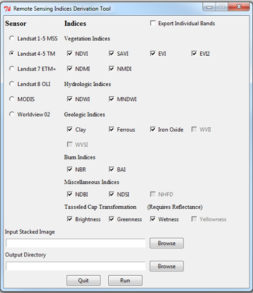
Figure 1. Remote Sensing Indices Derivation Tool GUI.

5. Run the tool and verify the output files visually in ArcMap v. 10.0 (ESRI, Redlands, CA) or another geographic information system software.

3. Software for Assisted Habitat Modeling (SAHM) (Figure 2)

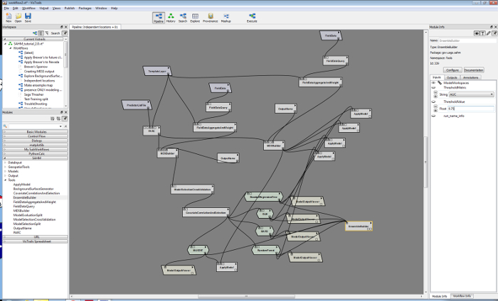
Figure 2. The entire SAHM workflow includes input data, preprocessing, preliminary model analysis and decision, correlative models, and output routines.

1. For running SAHM, first download files (including VisTrails) from the U.S. Geological Survey website at https://my.usgs.gov/catalog/RAM/SAHM. Refer to the User’s Guide at the same website for detailed instructions on downloading and installing SAHM. Note that the website also has a SAHM tutorial and data for additional instructions.
2. To develop the tamarisk species distribution models, use the SAHM_tutorial_2.0.vt file that comes with the package download (in the SAHM examples folder). Within the History view, select the Independent locations workflow. The other workflow examples can be selected and depend on study objectives; descriptions are provided with each. Select Pipeline.
3. Set the output folder, by going to Packages and then SAHM > Change Session Folder. Throughout the workflow development process, detailed descriptions of each step and options may be found by selecting the Documentation tab located on the right side of the SAHM viewer screen. All modules listed in the following methods can be found on the left side of the SAHM window under the SAHM tab.
4. Next, direct SAHM to the field data that will be used to train species distribution models.
   1. Click on the TemplateLayer module. Browse to the raster that will be used as a mask and to define the projection, cell size and extent of the analyses.
   2. Click on the FieldData module in the left side of the workflow. Browse to .csv (i.e., training.csv) file of field data (presence points or presence and absence points) within the field data module.
   3. Click on the PredictorListFile module and browse to .csv file list (e.g., file containing the full path to all predictors to use in the model- refer to user guide).
5. Next, conduct preprocessing steps.
   1. Click on the FieldDataQuery module and fill in response column with column heading for response (i.e., the column names in the FieldData.csv), X and Y columns.
   2. Click on the MDSBuilder module. Set the backgroundPointField to 10,000.
      NOTE: If you are using presence and absence data for the species being modeled, you do not need to change the backgroundPointField; you would include these locations with a response (0) in the Field Data.csv. It is optional to set a backgroundProbSurf if you want to constrain background point selection within an area by pointing to a raster surface with values ranging from 0 to 100 (these values represent the probability that a randomly generated point will be retained should it fall within a particular cell). For this study, use a backgroundProbSurf with values of 100 within a 5,000 m buffer of the Arkansas River and 0 for areas outside this buffer (based on the total area sampled by the tamarisk coalition).
6. Next, specify the species distribution modeling algorithms to be used.
   1. Note that the BoostedRegressionTree, GLM, MARS, and RandomForest modules are already set up in the Independent locations workflow. Add the MAXENT module to the workflow to test all five models. Connect it to the CovariateCorrelationAndSelection module.
      NOTE: Begin with default settings for all models; these can be modified based on study objectives (see model documentation for more details).
   2. Add a ModelOutputViewer module and connect it to the MAXENT module; change column to 5 and row to 1. The ModelOutputViewer produces a spreadsheet that can be used for model result comparisons.
   3. Click on the OutputName module and type a subfolder name.
7. Next, add a module that creates an ensemble of model outputs. This module produces two output maps; one with the average continuous probability of all the included outputs and a second with the count of the number of models with a positive binary probability.
   1. Add an EnsembleBuilder module to the workflow. It is optional to set a Threshold Metric; for this study, choose AUC and leave the Threshold Value at the default value of 0.75. This will ensure that only models with an AUC value greater than or equal to 0.75 are included in the ensemble map outputs. Connect the BoostedRegressionTree, GLM, MARS, RandomForest, and MAXENT modules to the EnsembleBuilder.
8. Next, direct the models to the independent test data.
   1. Click on the other FieldData module (right side of the workflow) and browse to the .csv file that contains model validation data. These are the 200 presence and absence points generated in step 1.4 of the PROTOCOL.
   2. Click on the FieldDataQuery module and make sure the response, x, and y columns match the columns in the field data .csv.
   3. Add an ApplyModel module and connect it to the MAXENT module. Add a ModelOutputViewer module and connect it to this ApplyModel module; change the column to 5 and the row to 1. In the menu, select Packages -> SAHM -> Change Processing Mode. Since you want to run more than one model, select single models sequentially (n - 1 cores each). This will expedite the execution time of the models by taking advantage of multiple computer cores.
9. Next, execute the species distribution models.
   1. Save the file .vt and then click on Execute.
   2. When the CovariateCorrelationAndSelection widget (Figure 3) appears, de-select one of each correlated pair of variables where the correlation coefficient is |r| ≥ 0.7 (based on % Deviance Explained from a univariate generalized additive model seen in on the left side of this widget (Figure 3) and informed ecological decisions; in this study prioritize the selection of at least one covariate for each month to capture phenological variation in tamarisk). The Number of Plots in the viewing window can be changed by typing in a number (the default is 8) and clicking on Update.
   3. After finalizing covariate selection, select OK at the bottom of the CovariateCorrelationAndSelection widget (Figure 3). For this study, the following 9 variables were retained: July_30_2006_Brightness, June_09_2005_SAVI, Sept_16_2006_SAVI, May_24_2005_B4, Oct_28_2004_NDVI, April_22_2005_Brightness, April_09_2006_SAVI, Aug_31_2006_B4, and Nov_19_2006_SAVI. The species distribution models will execute after selecting OK.

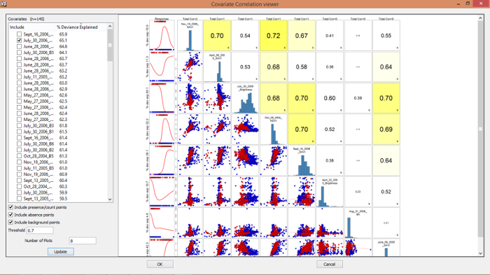
Figure 3. Covariate correlation and selection SAHM interface.

10. Results output.
    NOTE: After the models have completed, a VisTrails Spreadsheet appears for model comparison (Figure 4)
    1. Compare AUC plots, text outputs, response curves, calibration, confusion matrix, residuals, and response curves across models.
       NOTE: Output from SAHM models include a CovariateCorrelationOutputMDS, confusion matrix, residual plot, calibration plot, model evaluation plot, variable importance plot, a response curves folder, an expanded output folder, bin map, mess map, MoD map, prob map, residual map, and an output.txt; see the SAHM User Guide for more description.

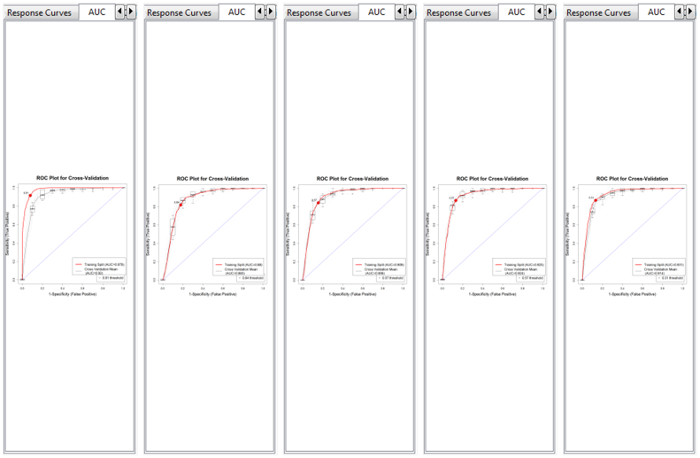
Figure 4. VisTrails spreadsheets can be used to evaluate model output. This is the AUC model comparison for the training data; from left to right the models are BRT, GLM, MARS, RF, and Maxent, respectively.

Results

Statistical evaluations of BRT, RF, MARS, GLM, and Maxent based on the independent test dataset indicated all five models performed relatively well in detecting tamarisk; there was little difference between threshold independent and threshold dependent evaluation metrics among models. AUC values were > 0.88, percent correctly classified values were > 77%, sensitivities and specificities were > 0.77, and TSS were > 0.54 (Table 1). An ensemble of binary model outputs revealed much model agreement in areas along the Arkansas River (Figure 5). The MESS (multivariate environmental similarity surface) map outputs for each model indicated the available environment of the study area was well sampled (Figure 6), further increasing our confidence in the ensemble approach.

Model	AUC	PCC	Sensitivity	Specificity	TSS
BRT	0.91	85	0.85	0.85	0.70
RF	0.92	85	0.85	0.85	0.70
MARS	0.90	82	0.82	0.82	0.64
GLM	0.88	77	0.77	0.77	0.54
Maxent	0.92	84	0.83	0.84	0.67

Table 1. Threshold independent (AUC) and threshold dependent (PCC, Sensitivity, Specificity, and TSS) evaluation metrics for BRT, RF, MARS, GLM, and Maxent models fit to an independent test dataset of tamarisk presence and absence.

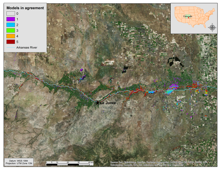
Figure 5. Ensemble results combining BRT, GLM, MARS, RF, and Maxent binary output maps in ArcGIS. Areas are colored by number of models in agreement, from 0 (no color) to 5 (red). Note the colored area in the northwest corner of the prediction; this line is an artifact of Landsat imagery; therefore model results should be taken with caution in this region. Please click here to view a larger version of this figure.

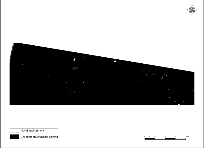
Figure 6. Multivariate environmental similarity surface (MESS) output. Please click here to view a larger version of this figure.

Of the nine predictors used, June 30 2006 Brightness was the most important variable for all five models (Table 2). This was the only variable retained by GLM based on stepwise Akaike information criterion (AIC; this is the default for GLM model selection in SAHM), however it is important to note this model also included a squared term of this variable. RF and Maxent retain all variables by default.

Predictor	BRT	RF	MARS	GLM	Maxent
July 30 2006 Brightness	41.60	34.11	76.78	100	67.27
August 31 2006 Band 4	6.35	5.87	5.16	0	2.82
June 09 2005 SAVI	13.67	14.09	9.14	0	9.75
April 22 2005 Brightness	6.29	6.30	0	0	0.43
October 28 2004 NDVI	5.66	8.25	0	0	2.94

Table 2. Relative importance of predictors in each model.

Discussion

Our results demonstrate fitting BRT, RF, MARS, GLM, and Maxent with presence points for tamarisk and a time-series of remotely sensed Landsat satellite imagery data can distinguish tamarisk on the landscape and is an effective alternative to traditional single-scene classification methods. It is clear from our results that June is a particularly important time for detecting tamarisk within our study area; this agrees with Evangelista et al. 2009¹ which indicated June Wetness was the most important predictor for tamarisk occurrence in this area based on a Maxent model fit with a time series of Landsat imagery.

The other spectral indices and bands that were included in the BRT, RF, MARS, and Maxent models may further distinguish tamarisk from soil substrate, other deciduous trees including cottonwood (Populus spp.) and willow (Salix spp.), or irrigated agriculture that is common in the lower Arkansas River basin. Other GIS layers, such as topography, soil types, or climate data could also be considered as covariates and included in these models, but we recommend keeping these to a minimum if the goal is to detect current species distribution on the landscape rather than predict potential occurrence or suitable habitat.

The models tested for our research provided strong analytical capacity and multiple options for evaluating results. Having all of these correlative models within a single framework, such as SAHM, allows the formalization and tractable recording of the modeling process. Pre- and post-processing of response and predictor variables are standardized in SAHM, allowing better and efficient model comparisons, while workflows record each step of the analyses facilitating modification, iteration and replication.

Ensemble mapping aims to combine the strengths of several correlative models, while minimizing the weakness of any one model³⁰. We believe this was the case in our study; however, we caution that models that underperform (i.e., under-predict or over-predict) can weaken the overall results. The limited use of ensemble mapping in the literature has had favorable results, but most of these approaches have attempted to "predict" species occurrence rather than "detect." Furthermore, ensemble mapping allows for a visual assessment of uncertainty among the different modeling methods, identifying levels of model agreement. Most often it is the choice of modeling method (e.g., GLM versus BRT) that has greatest quantifiable impact on model results rather than other decisions in the modeling process such as location data uncertainty³¹. Although we believe that our best tamarisk map is where all five models are in agreement, further testing and using various methods of ensemble mapping is recommended (e.g., weighted by AUC)³², and best validated through independent field observations. In summary, these methods can easily be tailored to model the distribution of other species using environmental variables derived for a given study region in SAHM.

Materials

List of materials used in this article

Name	Company	Catalog Number	Comments
Earth Explorer	USGS	http://earthexplorer.usgs.gov	Open Access: Yes
Remote Sensing Indices Derivation Tool	github	https://github.com/rander38/Remote-Sensing-Indices-Derivation-Tool	Open Access: Yes
Software for Assisted Habitat Modeling	USGS	https://my.usgs.gov/catalog/RAM/SAHM	Open Access: Yes
ArcGIS v.10.3	Esri	https://www.arcgis.com/features/	Open Access: No

References

- Evangelista, P. H., Stohlgren, T. J., Morisette, J. T., Kumar, S. Mapping invasive tamarisk (Tamarix): a comparison of single-scene and time-series analyses of remotely sensed data. Remote Sensing. 1, 519-533 (2009).
- DiTomaso, J. M. Impact, biology, and ecology of saltcedar (Tamarix spp.) in the southwestern United States. Weed Technology. 12, 326-336 (1998).
- Evangelista, P., Kumar, S., Stohlgren, T., Crall, A., Newman, G. Modeling above-ground biomass of Tamarisk ramosissima in the Arkansas River Basin of Southeastern Colorado, USA. Western North American Naturalist. 67 (4), 503-509 (2007).
- Hirano, A., Madden, M., Welch, R. Hyperspectral image data for mapping wetland vegetation. Wetlands. 23 (2), 436-448 (2003).
- Ge, S., Carruthers, R., Gong, P., Herrera, A. Texture analysis for mapping Tamarix pariviflora using aerial photographs along Cache Creek, California. Environmental Monitoring and Assessment. 114, 65-83 (2006).
- Hamada, Y., Stow, D. A., Coulter, L. L., Jafolla, J. C., Hendricks, L. W. Detecting tamarisk species (Tamarisk spp.) in riparian habitats of Southern California using high spatial resolution hyperspectral imagery. Remote Sensing of Environment. 109, 237-248 (2007).
- York, P., Evangelista, P., Kumar, S., Graham, J., Flather, C., Stohlgren, T. A Habitat Overlap Analysis derived from Maxent for Tamarisk and the Southwestern Willow Flycatcher. Frontiers of Earth Science. 5 (2), 120-129 (2011).
- Myneni, R. B., Ramakrishna, R., Nemani, R., Running, S. W. Estimation of global leaf area index and absorbed par using radiative transfer models. Geoscience and Remote Sensing. 35 (6), 1380-1393 (1997).
- Todd, S. W., Hoffer, R. M., Milchunas, D. G. Biomass estimation on grazed and ungrazed rangelands using spectral indices. International Journal of Remote Sensing. 19 (3), 427-438 (1998).
- Rouse, J. W., Haas, R. H., Schell, J. A., Deering, D. W. Monitoring vegetation systems in the Great Plains with ERTS. Proceedings of the Third Earth Resources Technology Satellite-1 Symposium. , (1974).
- Huete, A. R. A Soil-Adjusted Vegetation Index (SAVI). Remote Sensing of Environment. 25, 295-309 (1988).
- Kauth, R. J., Thomas, G. S. The tasselled cap - a graphic description of the spectral-temporal development of agricultural crops as seen in Landsat. Proceedings of the Symposium on Machine Processing of Remotely Sensed Data. , LARS, Purdue University. West Lafayette, Indiana. 41-51 (1976).
- Cohen, W. B., Spies, T. A., Fiorella, M. Estimating the age and structure of forests in a multi-ownership landscape of western Oregon, USA. International Journal of Remote Sensing. 16, 721-746 (1995).
- Jin, S., Sader, S. Comparison of time series tasselled cap wetness and the normalized difference moisture index in detecting forest disturbances. Remote Sensing of Environment. 94 (3), 364-372 (2005).
- Crist, E. P. A TM Tasseled Cap equivalent transformation for reflectance factor data. Remote Sensing of Environment. 17 (3), 301-306 (1985).
- Lindauer, I. E. A comparison of the plant communities of the South Platte and Arkansas River drainages in eastern Colorado. The Southwestern Naturalist. 28 (3), 249-259 (1983).
- Riparian Restoration: Assessment of alternative technologies for tamarisk control, biomass reduction and revegetation. , Tamarisk Coalition. Available from: http://www.tamariskcoalition.org (2008).
- Guisan, A., Zimmerman, N. Predictive habitat distribution models in ecology. Ecological Modeling. 135, 147-186 (2000).
- Friedman, J. H., Hastie, T., Tibshirani, R. Additive logistic regression: a statistical view of boosting. Annals of Statistics. 28 (2), 337-407 (2000).
- Breiman, L. Random forests. Machine Learning. 45 (1), 5-32 (2001).
- Friedman, J. H. Multivariate adaptive regression splines. Annals of Statistics. 19 (1), 1-141 (1991).
- McCullagh, P., Nelder, J. A. Generalized Linear Models, 2nd ed. , Chapman and Hall. London. (1989).
- Phillips, S. J., Anderson, R. P., Schapire, R. E. Maximum entropy modeling of species geographic distributions. Ecological Modelling. 190 (3-4), 231-259 (2006).
- Araujo, M. B., New, M. Ensemble forecasting of species distributions. Trends in Ecology and Evolution. 22, 42-47 (2007).
- Elith, J., Graham, C. H. Do they? How do they? Why do they differ? On finding reasons for differing performances of species distribution models. Ecography. 32, 66-77 (2009).
- Freire, J., Silva, C., Callahan, S., Santos, E., Schedegger, C. Managing rapidly-evolving scientific workflows. International Provenance and Annotation Workshop (IPAW). Moreau, L., Foster, I. , Springer. 10-18 (2006).
- Morisette, J. T., Jarnevich, C. S., Holcombe, T. R., Talbert, C. B., Ignizio, D., Talbert, M. K., et al. VisTrails SAHM: visualization and workflow management for species habitat modeling. Ecography. 36 (2), 129-135 (2013).
- Fielding, A. H., Bell, J. F. A review of methods for the assessment of prediction errors in conservation presence/absence models. Environmental Conservation. 24, 38-49 (1997).
- Allouche, O., Tsoar, A., Kadmon, R. Assessing the accuracy of species distribution models: prevalence, kappa and the true skill statistic (TSS). Journal of Applied Ecology. 43 (6), 1223-1232 (2006).
- Stohlgren, T. J., Ma, P., Kumar, S., Rocca, M., Morisette, J., Jarnevich, C. S. Ensemble habitat mapping of invasive plant species. Risk Analysis. 30, 224-235 (2010).
- Dormann, C. F., Purschke, O., Marquez, J. R. G., Lautenbach, S., Schrader, B. Components of uncertainty in species distribution analysis: A case study of the great grey shrike. Ecology. 89, 3371-3386 (2008).
- Marmion, M., Parviainen, M., Luoto, M., Heikkinen, R. K., Thuiller, W. Evaluation of consensus methods in predictive species distribution modelling. Diversity and Distributions. 15, 59-69 (2009).
Reprints and Permissions