Preparation of Liquid-exfoliated Transition Metal Dichalcogenide Nanosheets with Controlled Size and Thickness: A State of the Art Protocol

Summary

A protocol for the liquid exfoliation of layered materials to nanosheets, their size selection and size measurement by microscopic and spectroscopic techniques is presented.

Abstract

We summarize recent advances in the production of liquid-exfoliated transition metal dichalcogenide (TMD) nanosheets with controlled size and thickness. Layered crystals of molybdenum disulphide (MoS₂) and tungsten disulphide (WS₂) are exfoliated in aqueous surfactant solution by sonication. This yields highly polydisperse mixtures containing nanosheets with broad size and thickness distributions. However, for most purposes, specific sizes (in terms of both lateral dimension and thickness) are required. For example, large and thin nanosheets are desired for (opto) electronic applications, while laterally small nanosheets are interesting for catalytic applications. Therefore, post-exfoliation size selection is an important step that we address here. We provide a detailed protocol on the efficient size selection in large quantities by liquid cascade centrifugation and the size and thickness quantification by statistical microscopic analysis (atomic force microscopy and transmission electron microscopy). The comparison of MoS₂ and WS₂ shows that both materials are size-selected in a similar way by the same procedure. Importantly, the dispersions of size-selected nanosheets show systematic changes in their optical extinction spectra with size due to edge and confinement effects. We show how these optical changes are related quantitatively to the nanosheets dimensions and describe how mean nanosheets length and layer number can be extracted reliably from the extinction spectra. The exfoliation and size selection protocol can be applied to a broad range of layered crystals as we have previously demonstrated for graphene, gallium sulphide (GaS) and black phosphorus.

Introduction

The possibility to produce and process graphene, related two-dimensional (2D) crystals in the liquid phase makes them promising materials for an ever growing range of applications as composite materials, sensors, in energy storage and conversion and flexible (opto) electronics.^1-6 To exploit 2D nanomaterials within applications such as these will require inexpensive and reliable functional inks with on-demand lateral size and thickness of the nanoscale constituents, as well as controlled rheological and morphological properties amenable to industrial-scale printing/coating processes.⁷ In this regard, liquid phase exfoliation has become an important production technique giving access to a whole host of nanostructures in large quantities.^6,8,9 This method involves the sonication or shearing of layered crystals in liquids. If the liquid is appropriately chosen (i.e., suitable solvents or surfactant) the nanosheets will be stabilized against reaggregation. Numerous applications and proof-of-principle devices have been demonstrated by such techniques.⁶ Probably the greatest strength of this strategy is its versatility, as numerous layered parent crystals can be exfoliated and processed in a similar way, providing access to a broad palette of materials which can be tailored to the desired application.

However, despite this recent progress, the resultant polydispersity that arises due to these liquid-phase production methods (in terms of nanosheet length and thickness) still presents a bottleneck in the realization of high performance devices. This is mostly because the development of novel and innovative size selection techniques has thus far required nanosheets length and thickness characterization using tedious statistical microscopy (atomic force microscopy, AFM and/or transmission electron microscopy, TEM).

Despite these challenges, several centrifugation techniques have been reported to achieve length and thickness sorting.^6,10-13 The simplest scenario is homogeneous centrifugation, where the dispersion is centrifuged at a given centrifugal acceleration and the supernatant is decanted for analysis. The centrifugation speed sets the size cut-off, whereby the higher the speed, the smaller are the nanosheets in the supernatant. However, this technique suffers from two major disadvantages; firstly, when larger nanosheets are to be selected (i.e., the dispersion is centrifuged at low speeds and the supernatant is decanted) all smaller nanosheets will also remain in the sample. Secondly, regardless of the centrifugation speed, a significant proportion of the material tends to be wasted in the sediment.

An alternative strategy for size selection is density gradient (or isopycnic) centrifugation.^11,14 In this case, the dispersion is injected into a centrifuge tube containing a density gradient medium. During ultracentrifugation (typically > 200,000 x g), a density gradient is formed and the nanosheets move to the point in the centrifuge where their buoyant density (density including the stabilizer and solvent shell) matches the density of the gradient. Note that the nanomaterial can also move upward during this process (depending on where it was injected). In such a way, the nanosheets are effectively sorted by thickness rather than mass (opposed to homogeneous centrifugation). While this procedure offers a unique opportunity to sort nanosheets by thickness, it suffers from notable disadvantages. For example, the yields are very low and at present do not allow for the mass production of separated nanosheets. This is partly related to low contents of monolayers in stock dispersions after liquid-exfoliation and can potentially be improved by optimizing exfoliation procedures in the future. In addition, it is typically a time-consuming multi-step ultracentrifugation process involving multiple iterations to achieve efficient size selection. Furthermore, in the case of inorganic nanomaterials, it is restricted to polymer-stabilized dispersions to obtain the required buoyant densities and the gradient medium in the dispersion may interfere with further processing.

We have recently shown that a procedure we term liquid cascade centrifugation (LCC) offers an exciting alternative,¹³ as we will also detail in this manuscript. This is a multi-step procedure which is extremely versatile allowing various cascades to be designed according to the desired outcome. To demonstrate this process, a standard cascade is portrayed in Figure 1 and involves multiple centrifugation steps whereby each features a higher speed than the last. After each step, the sediment is retained and the supernatant is then used in the proceeding stage. As a result, each sediment contains nanosheets in a given size range which have been "trapped" between two centrifugations with different speeds; the lower one removing larger nanosheets into the previous sediment while the higher speed removes the smaller nanosheets into the supernatant. Critical to LCC, the resulting sediment can be redispersed completely by mild sonication in the respective medium, which in this case is aqueous sodium cholate H₂O-SC (at SC concentrations as low as 0.1 g L^-1). The result is dispersions with virtually any chosen concentration. Importantly, virtually no material is wasted in LCC, resulting in the collection of relatively large masses of size-selected nanosheets. As shown here, we have applied this procedure to a number of liquid-exfoliated nanosheets including MoS₂ and WS₂ as well as GaS,¹⁵ black phosphorus¹⁶ and graphene¹⁷ in both solvent and surfactant systems.

This unique centrifugation procedure enables the efficient size-selection of liquid exfoliated nanosheets and has subsequently enabled a significant advancement in terms of their size and thickness determination. In particular, through this approach we demonstrated previously that optical extinction (and absorbance) spectra of the nanosheets change systematically as function of both nanosheets lateral dimensions and nanosheets thickness. As we summarize here, this has allowed us to link the nanosheet spectral profile (specifically the intensity ratio at two positions of the extinction spectrum) to the mean nanosheet length as a result of nanosheet edge effects.^12,13 Importantly, the same equation can be used to quantify the size of MoS₂ and WS₂. Furthermore, we show that the A-exciton position shifts towards lower wavelengths as a function of mean nanosheet thickness due to confinement effects. Even though exfoliation, as well as size selection and determination are in general rather robust procedures, the quantitative outcome depends on subtleties in the protocol. However, especially for newcomers to the field, it is difficult to judge which process parameters are most relevant. This comes down to the fact that experimental sections of research papers only provide a rough protocol, without discussing what outcome is to be expected when modifying the procedure or giving a rational behind the protocol. In this contribution, we intend to address this as well as provide a detailed guide and discussion to the production of liquid-exfoliated nanosheets of controlled size and to the accurate determination of size by either statistical microscopy or analysis of the extinction spectra. We are convinced that this will help to improve reproducibility and hope it will be a useful guide for other experimentalists in this research area.

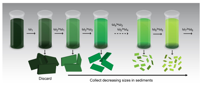
Figure 1: Schematic of the size selection by liquid cascade centrifugation. Size-selected nanosheets are collected as sediments. Each sediment is collected or "trapped" between two centrifugation speeds (ω) starting from low speeds and going to higher ones from step to step. The sediment discarded after the first centrifugation contains unexfoliated layered crystallites while the supernatant discarded after the last centrifugation step contains extremely small nanosheets. Size-selected dispersions are prepared by re-dispersing the collected sediments in the same medium (here aqueous surfactant solution) at reduced volumes. Adapted with permission from ¹³. Please click here to view a larger version of this figure.

Protocol

1. Liquid Exfoliation — Preparation of Suitable Stock Dispersions

1. Mount a metal cup underneath a sonotrode in an ice bath.
2. Immerse 1.6 g of the TMD powder in 80 mL aqueous solution of sodium cholate (SC) surfactant (sodium cholate concentration, C_SC= 6 g L^-1) in the metal cup.
3. Move the sonic tip to the bottom of the metal cup and then up by ~ 1 cm. Wrap aluminum foil around the sonic probe to avoid spillage.
4. Sonicate the mixture under ice-cooling by probe sonication to avoid heating using a solid flathead tip (750 W processor) for 1 h at 60% amplitude (pulse of 6 s on and 2 s off).
5. Centrifuge the dispersion at a centrifugation speed of 2,660 x g for 1.5 h. Discard the supernatant containing impurities and collect the sediment in 80 mL fresh surfactant solution (C_SC= 2 g L^-1).
   NOTE: Use maximum filling heights in the centrifuge tubes of maximum 10 cm. Otherwise, increase the centrifugation time.
6. Subject the dispersion to a second, longer sonication using the solid flathead tip for 5 h at 60% amplitude (pulse of 6 s on and 2 s off) under ice-cooling. Replace the ice bath every 2 h while pausing the sonication.

2. Nanosheet Size Selection by Liquid Cascade Centrifugation

NOTE: To select nanosheets by size, liquid cascade centrifugation with sequentially increasing centrifugal acceleration is applied (Figure 1). The following procedure is recommended as standard size selection of the cascade in the case of TMDs. For other materials, centrifugation speeds may need to be adjusted.

1. Remove unexfoliated powder by centrifugation at 240 x g (1.5 krpm), 2 h. Discard the sediment.
2. Centrifuge the supernatant at a higher centrifugal acceleration: 425 x g (2 krpm), 2 h. Collect the sediment in fresh surfactant at reduced volume (3-8 mL).
3. Centrifuge the supernatant at even higher centrifugal acceleration: 950 x g (3 krpm), 2 h. Collect the sediment in fresh surfactant at reduced volume (3-8 mL).
4. Repeat this procedure with the following centrifugal accelerations: 1,700 x g (4 krpm), 2,650 x g (5 krpm), 3,500 x g (6 krpm), 5,500 x g (7.5 krpm), and 9,750 x g (10 krpm).

3. Determination of Nanosheets Size and Thickness by Statistical Microscopy

NOTE: If spectroscopic metrics are already available, section 3 can be skipped or reduced, i.e., not carried out for every sample.

1. Length: Transmission electron microscopy (TEM)
   1. Deposition
      1. Dilute the high concentration dispersions with water (to reduce the surfactant concentration) so that they are of light in color. Drop cast onto a grid (for example holey carbon, 400 mesh) placed on a filter membrane to wick away excess solvent.
   2. Imaging
      1. Record multiple images on different positions on the grid. Adjust the field of view depending on nanosheet size. For a comprehensive TEM imaging tutorial, see reference ¹⁸.
   3. Statistical length analysis performed using ImageJ
      1. Open the ImageJ software, select the relevant TEM image via the "file" menu and "open" the image. The image will open in a new window.
      2. Click the "analyze" tab. Select "set scale" from the drop down menu. A new window will open. Click "remove scale", tick "global" and click "ok".
      3. Select the "line" tool. Draw a line profile along the length of the scale bar of the TEM image.
      4. Click "analyze". Select "set scale" from the drop down menu. Enter the length of the scale bar in nm into the "known distance" box and click "ok".
         NOTE: The distance of the line drawn on the scale bar is displayed in pixels.
      5. Select the "line" tool and measure the nanosheet length by drawing a line profile of the longest axis of the nanosheet.
      6. Press "control+M" to measure. A new box labelled "results" opens with the nanosheet length displayed in the "length" column.
      7. Repeat step 3.1.3.6 for all individually deposited nanosheets (not aggregated ones) in the image.
      8. When opening a new image, repeat steps 3.1.3.3- 3.1.3.7. Count the length of 150 nanosheets.
         NOTE: All nanosheet length data is compiled in the "results" window and can be copied into other programs for further processing.
2. Thickness: Atomic force microscopy (AFM)
   1. Dilute the dispersion so that are almost transparent to the human eye (corresponding to extinction intensity of ideally ~0.2 per 1 cm pathlength at 400 nm). In the case of surfactant dispersions, dilute with water not surfactant.
   2. Drop-cast on pre-heated wafers. For water-based dispersion, heat the wafer to ~170 °C on a hot plate and deposit 10 µL per 0.5 x 0.5 cm² wafer.
   3. Rinse the wafers thoroughly with a minimum of 5 mL of water and 3 mL of 2-propanol to remove residual surfactant and other impurities.
   4. Scan and save multiple images across the sample with the AFM in tapping mode. For small nanosheets use a resolution of 512 lines per image and image sizes of maximum 2 x 2 µm². For samples containing larger nanosheets, increase the field of view to up to 8 x 8 µm². Use scan rates as appropriate (typically 0.4-0.7 Hz). Alternatively, scan larger areas at higher resolution.
   5. Thickness measurement using Gwyddion Software
      1. Open the software and select the relevant AFM image via "file" and "open". The image will open in a new window.
      2. Correct the background using the "level data by mean plane subtraction" "align rows" and "correct horizontal scars" in the "Data Process" section of the home menu. Apply the corrections, change the image color for better contrast by right-clicking on the legend and set z-plane to zero.
      3. Zoom in the region of choice (if convenient). Click on the "crop" tool in the home menu. Drag the cursor over the image to mark the region of choice. Press "apply". Check the "create new channel" to open the selected region in a new window.
      4. Select "extract profiles" from the tools menu. A new window opens.
      5. Draw a line across the nanosheet. Write down the thickness in a table. In the case of non-homogeneously thick nanosheets, average the thickness across the nanosheet. Take extreme care to measure only individually deposited and non-aggregated nanosheets.
      6. Repeat 3.2.5.3-3.2.5.5 for all nanosheets on the image.
      7. Repeat 3.2.5.1-3.2.5.6 for all images recorded. Count minimum 150 nanosheets.
3. Conversion of AFM thickness to layer number
   NOTE: Apparent AFM heights from liquid exfoliated nanomaterials are usually overestimated due to the presence of residual solvent. In addition, accurate height measurements of inhomogeneous samples (such as nanomaterials deposited on substrates) using AFM are generally challenging due to contributions from effects such as capillary forces and adhesion which depend on the material and measurement parameters.^19,20 To overcome these problems and to convert the apparent measured AFM thickness to the number of layers, a procedure termed step height analysis was developed as described in the following.^12,13,16,21. Steps 3.3.1-3.3.4 can be skipped if the step height is known.
   1. Open, correct and crop the AFM image as described in 3.2 to select a nanosheet with clearly discernible terraces.
   2. Measure the height across the nanosheet using the "extract" profile tool.
      NOTE: Suitable profiles show discrete steps as the one in Figure 2B inset.
      1. Record the height of these steps (i.e., the height difference from one terrace to the next on the nanosheet).
   3. Count at least 70 of these steps.
   4. Plot the step height in ascending order (Figure 2C).
      NOTE: Observe that for TMDs the apparent step height is always a multiple of ~1.9 nm.
   5. Divide the apparent AFM thickness (measured as described in section 3.2) by 1.9 nm to obtain the layer number.
      NOTE: Other materials have other step height conversion factors requiring a different calibration.

4. Determination of MoS₂ and WS₂ Size and Thickness Based on Extinction Spectra

1. Spectra acquisition
   1. Dilute the high concentration samples with the respective medium (here aqueous sodium cholate, 2 g L^-1) to yield extinctions below 2 across the entire spectral range.
   2. Set the increments for the spectral acquisition to 0.5 nm in the instrument settings or use scan speed slow or medium.
   3. Choose the settings "subtract baseline" in the instrument settings. Place the cuvette containing the aqueous sodium cholate solution in the sample compartment of the spectrometer and run the measurement.
   4. Remove the cuvette with the sodium cholate solution from the spectrometer and empty it. Fill in the sample, place the sample in the sample compartment of the spectrometer and run a scan of the sample.
2. Length determination from intensity ratios
   1. Option 1: Read-off the intensity at the A-exciton, Ext_A (~660 nm for MoS₂ and 620 nm for WS₂) and the local minimum Ext_min (345 nm for MoS₂ and 295 nm for WS₂). Divide the intensity at the A-exciton by the intensity at the local minimum to obtain the intensity ratio Ext_A/Ext_min.
   2. Determine the mean nanosheet length, by using equation 1.
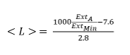      (Eq. 1)
      where Ext_A/Ext_min is the intensity ratio of the extinction at the A-exciton (Ext_A) and the local minimum (Ext_min).
      NOTE: The equation holds for both MoS₂ and WS₂. However, its accuracy is limited especially for small nanosheets.
   3. Option 2: Determine the intensity ratio of the local maximum in the UV region of the spectrum, Ext_Max-HE (270 nm for MoS₂ and 235 nm for WS₂) and the local minimum, Ext_min (345 nm for MoS₂ and 295 nm for WS₂)
   4. Determine the mean nanosheet length, by using equation 2.
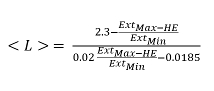      (Eq. 2)
      With Ext_max-HE denoting the intensity at the local maximum at high energy (270 nm for MoS₂ and 235 nm for WS₂) and Ext_min the extinction intensity at the local minimum (345 nm for MoS₂ and 295 nm for WS₂).
      NOTE: Option 2 gives a more accurate measure of the lateral size. However, the high energy region may not be accessible in all solvents/surfactant.
3. Concentration
   1. Record the extinction intensity relative to 1 cm pathlength at 345 nm for MoS₂ and 235 nm for WS₂, respectively.
      NOTE: Divide the recorded measured extinction by the pathlength of the cuvette.
   2. Divide this intensity by the extinction coefficients of 68 Lg^-1cm^-1 at 345 nm for MoS₂ and 47 Lg^-1cm^-1 at 235 nm for WS₂ to obtain the nanosheet concentration in gL^-1.
4. Thickness determination from A-exciton position
   1. Calculate the second derivative of the spectrum.
      1. Using the data analysis and graphing software (e.g., OriginPro), select the column containing the extinction intensity. Click on the "analysis" tab, select "mathematics" from the drop down menu and "differentiate", "open dialog". A new window will open. Set the derivative order to 2 and press ok.
   2. Smooth the second derivative by Adjacent Averaging (~ 10-20 points per window in A-exciton region).
      1. For example, using the data analysis and graphing software, plot the second derivative spectrum.
         1. With the graphic window active, click on "analysis" and choose "signal processing", then "smooth" then "open dialog" from the drop down menu. A new window will open.
         2. Choose "Adjacent Averaging" as smoothing method and set the points to 20.
         3. Plot the resultant smoothed spectrum which is displayed as new columns. If the noise is still high, repeat the smoothing.
            NOTE: Usually, spectral smoothing is required to reduce the noise unless high integration times during the measurement are used. The appropriate smoothing is an important part of the data analysis and the appropriate smoothing method depends on the desired outcome. This particular smoothing method is only ideal to determine the mean peak position.¹³
   3. Read-off the peak position from the second derivative. This is the wavelength of the A-exciton, λ_A. Alternatively, carry out the steps described in 4.4.4-4.4.7.
   4. Convert the x-axis from wavelength to energy using the relation:
      E(eV) = 4.135E-6 * 2.997E8 / λ(nm)
   5. Fit the second derivative to the second derivative of a Lorentzian.
      NOTE: A Lorentzian can be written as
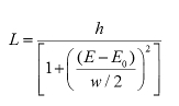      (Eq. 3)
      Where h is the height, E'₀ is the center and w is the FWHM. Differentiating twice with respect to E gives
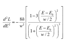      (Eq. 4)
      1. In the data analysis and graphing software, choose "tools" from the main menu and select "fitting function builder". A new window will open.
      2. Select "create a new function", click next.
      3. Leave the default settings, give the function a name and click next.
      4. Set "h,E,w" as parameters, click next.
      5. Enter "(-8*h/w^2)*(1-3*(2*(E-x)/w)^2)/(1+(2*(E-x)/w)^2)^3" as function body, click finish.
      6. Plot only the A-exciton region of the second derivative spectrum on the energy scale.
      7. With the graphics window active, click on the "analysis" tab. Choose "fitting", "nonlinear curve fit", "open dialog" from the drop down menu. A new window will open.
      8. Select "user defined" in category and choose the previously built function in the function box. In the tab "parameters" set initial values for w to 0.1, and E to 1.99 for WS₂ and 1.85 for MoS₂. Press "fit"
   6. Record the energy E'₀, which is the energy associated with the A-exciton, E'_A.
   7. Determine the number of layers according to equations 5 (MoS₂) and 6 (WS₂).
      (Eq. 5, MoS₂)
      (Eq. 6, WS₂)
      with λ_A denoting the wavelength of the A-exciton and E_A denoting the energy of the A-exciton.

Results

Liquid cascade centrifugation (Figure 1) is a powerful technique to sort liquid-exfoliated nanosheets by size and thickness as illustrated in Figure 2 for both MoS₂ and WS₂. Nanosheet lateral sizes and thicknesses can be characterized by statistical TEM and AFM, respectively. A typical AFM image is shown in Figure 2A. The apparent nanosheet thickness is converted to layer number using step height analysis (Fi...

Discussion

Sample preparation

The samples described here are produced by tip sonication. Alternative exfoliation procedures can be used, but will lead to different concentrations, lateral sizes and degrees of exfoliation. Higher amplitudes and longer on pulses during the sonication should be avoided to prevent damaging of the sonicator. Similar results were obtained using 500 W processors. However, sonication time and amplitude has an impact on the nanosheet exfoliation and variations from this protocol may...

Materials

List of materials used in this article

Name	Company	Catalog Number	Comments
Sodium cholate hydrate, from ox and/or sheep bile	Sigma Aldrich	C1254-100G	Surfactant used as stabilizer in the form of an aqueous solution (i.e., after dissolving the powder in millipore water)
MoS2 powder	Sigma Aldrich	69860-100G	Other distributors available, but exfoliation and outcome of size selection can vary
WS2, powder 2 μm	Sigma Aldrich	243639-50G	Other distributors available, but exfoliation and outcome of size selection can vary
ImageJ Software	Developer: National Insitutes of Health	64-bit Java version 2.45 1.6.0_24	Image processing software used for TEM analysis, free download
Gwyddion Software	Developer: Czech Metrology Institute	64-bit Java version 2.45	Image processing software used for AFM analysis, free download
Origin Pro Software	OriginLab	Version 2016	Software used for data analysis such as differntiation and fitting of the extinction spectra
Centrifuge	HettichLab	Mikro 220R	any other benchtop centrifuge is suitable
Rotor 1	Hettich	Rotor 1016	for centrifugation <5,000 x g
Rotor 2	Hettich	Rotor 1195-A	for centrifugation >5,000 x g

References

- Zhang, H. Ultrathin Two-Dimensional Nanomaterials. ACS Nano. 9, 9451-9469 (2015).
- Yi, M., Shen, Z. A review on mechanical exfoliation for the scalable production of graphene. J. Mat. Chem. A. 3, 11700-11715 (2015).
- Jariwala, D., Sangwan, V. K., Lauhon, L. J., Marks, T. J., Hersam, M. C. Emerging Device Applications for Semiconducting Two-Dimensional Transition Metal Dichalcogenides. ACS Nano. 8, 1102-1120 (2014).
- Nicolosi, V., Chhowalla, M., Kanatzidis, M. G., Strano, M. S., Coleman, J. N. Liquid Exfoliation of Layered Materials. Science. 340, 1420(2013).
- Butler, S. Z., et al. Progress, Challenges, and Opportunities in Two-Dimensional Materials Beyond Graphene. ACS Nano. 7, 2898-2926 (2013).
- Bonaccorso, F., Bartolotta, A., Coleman, J. N., Backes, C. Two-dimensional crystals-based functional inks. Adv. Mater. , accepted (2016).
- Torrisi, F., Coleman, J. N. Electrifying inks with 2D materials. Nat. Nanotechnol. 9, 738-739 (2014).
- Coleman, J. N., et al. Two-Dimensional Nanosheets Produced by Liquid Exfoliation of Layered Materials. Science. 331, 568-571 (2011).
- Smith, R. J., et al. Large-Scale Exfoliation of Inorganic Layered Compounds in Aqueous Surfactant Solutions. Adv. Mater. 23, 3944-3948 (2011).
- Khan, U., O'Neill, A., Porwal, H., May, P., Nawaz, K., Coleman, J. N. Size selection of dispersed, exfoliated graphene flakes by controlled centrifugation. Carbon. 50, 470-475 (2012).
- Kang, J., Seo, J. -W. T., Alducin, D., Ponce, A., Yacaman, M. J., Hersam, M. C. Thickness sorting of two-dimensional transition metal dichalcogenides via copolymer-assisted density gradient ultracentrifugation. Nat. Commun. 5, 5478(2014).
- Backes, C., et al. Edge and Confinement Effects Allow in situ Measurement of Size and Thickness of Liquid-Exfoliated Nanosheets. Nat. Commun. 5, 4576(2014).
- Backes, C., et al. Production of Highly Monolayer Enriched Dispersions of Liquid-Exfoliated Nanosheets by Liquid Cascade Centrifugation. ACS Nano. 10, 1589-1601 (2016).
- Green, A. A., Hersam, M. C. Solution Phase Production of Graphene with Controlled Thickness via Density Differentiation. Nano Lett. 9, 4031-4036 (2009).
- Harvey, A., et al. Preparation of Gallium Sulfide Nanosheets by Liquid Exfoliation and Their Application As Hydrogen Evolution Catalysts. Chem. Mater. 27, 3483-3493 (2015).
- Hanlon, D., et al. Liquid Exfoliation of Solvent-Stabilised Few-Layer Black Phosphorus for Applications Beyond Electronics. Nat. Commun. 6, 8563(2015).
- Backes, C., et al. Spectroscopic metrics allow in-situ measurement of mean size and thickness of liquid-exfoliated few-layered graphene nanosheets. Nanoscale. 8, 4311-4323 (2016).
- Rodenburg, J. Tutorial Courses on Transmission Electron Microscopy. , Available from: http://www.rodenburg.org/ (2016).
- Ridings, C., Warr, G. G., Andersson, G. G. Composition of the outermost layer and concentration depth profiles of ammonium nitrate ionic liquid surfaces. Phys. Chem. Chem. Phys. 14, 16088-16095 (2012).
- Nemes-Incze, P., Osváth, Z., Kamarás, K., Biró, L. P. Anomalies in thickness measurements of graphene and few layer graphite crystals by tapping mode atomic force microscopy. Carbon. 46, 1435-1442 (2008).
- Paton, K. R., et al. Scalable production of large quantities of defect-free few-layer graphene by shear exfoliation in liquids. Nat. Mater. 13, 624-630 (2014).
- Novoselov, K. S., et al. Two-dimensional atomic crystals. Proc. Nat. Ac. Sci. U. S. 102, 10451-10453 (2005).
- Kouroupis-Agalou, K., et al. Nanoscale. 6, 5926-5933 (2014).
- Hanlon, D., et al. Production of Molybdenum Trioxide Nanosheets by Liquid Exfoliation and Their Application in High-Performance Supercapacitors. Chem. Mater. 26, 1751-1763 (2014).
- Yadgarov, L., et al. Dependence of the Absorption and Optical Surface Plasmon Scattering of MoS2 Nanoparticles on Aspect Ratio, Size, and Media. ACS Nano. 8, 3575-3583 (2014).
- Wilson, J. A., Yoffe, A. D. Transition metal dichalcogenides. Discussion and interpretation of the observed optical, electrical, and structural properties. Adv. Phys. 18, 193-335 (1969).
Access restricted. Please log in or start a trial to view this content.
Reprints and Permissions