A Rapid Laser Probing Method Facilitates the Non-invasive and Contact-free Determination of Leaf Thermal Properties

Summary

A method was developed to determine the specific heat capacity and thermal conductivity of leaf tissue by non-invasive, contact-free near infrared laser probing, which requires less than 1 min per sample.

Abstract

Plants can produce valuable substances such as secondary metabolites and recombinant proteins. The purification of the latter from plant biomass can be streamlined by heat treatment (blanching). A blanching apparatus can be designed more precisely if the thermal properties of the leaves are known in detail, i.e., the specific heat capacity and thermal conductivity. The measurement of these properties is time consuming and labor intensive, and usually requires invasive methods that contact the sample directly. This can reduce the product yield and may be incompatible with containment requirements, e.g., in the context of good manufacturing practice. To address these issues, a non-invasive, contact-free method was developed that determines the specific heat capacity and thermal conductivity of an intact plant leaf in about one minute. The method involves the application of a short laser pulse of defined length and intensity to a small area of the leaf sample, causing a temperature increase that is measured using a near infrared sensor. The temperature increase is combined with known leaf properties (thickness and density) to determine the specific heat capacity. The thermal conductivity is then calculated based on the profile of the subsequent temperature decline, taking thermal radiation and convective heat transfer into account. The associated calculations and critical aspects of sample handling are discussed.

Introduction

The large-scale processing of biological materials often requires heat-treatment steps such as pasteurization. The equipment for such processes can be designed more precisely if the thermal properties of the biological materials are well characterized, including the specific heat capacity (c_p,s) and thermal conductivity (λ). These parameters can be determined easily for liquids, suspensions and homogenates by calorimetry ¹. However, measuring such parameters in solid samples can be labor intensive, and often requires direct contact with the sample or even its destruction ². For example, photothermal techniques require direct contact between the sample and detector ³. Such limitations are acceptable during food processing, but are incompatible with highly regulated processes such as the production of biopharmaceutical proteins in plants in the context of good manufacturing practice ⁴. In such a context, repeated (e.g., weekly) monitoring of thermal properties may be required during a seven-week growth period for individual plants as a quality control tool. If such a monitoring would require and consume a leaf for each measurement, there would be no biomass left to process at the time of harvest.

Additionally, using only leaf parts instead would cause wounding to the plant and increase the risk of necrosis or pathogen infection, again diminishing the process yield. The likelihood of pathogen infection may also increase if a method with direct contact to the sample would be used, inducing the risk that an entire batch of plants can be infected through contact with a contaminated sensor device. Similar aspects have to be considered for the monitoring of plant stresses like drought, e.g., in an ecophysiological context. For example, water loss is often monitored by a change in the fresh biomass, which requires an invasive treatment of the plants under investigation ⁵, e.g., dissecting a leaf. Instead, determining the specific heat capacity, which depends on the water content of a sample, in a non-invasive manner as describe here, can be used as a surrogate parameter for the hydration status of plants. In both scenarios (pharmaceutical production and ecophysiology), artificial stresses induced by destructive or invasive measurement techniques would be deleterious as they can distort the experimental data. Therefore, previously reported flash methods ⁶ or the placement of samples between silver plates ⁷ are unsuitable for such processes and experiments because they either require direct contact to the sample or are destructive. The parameters c_p,s and λ must be determined in order to design the process equipment for a blanching step that can simplify product purification and thus reduce manufacturing costs ^8-10. Both c_p,s and λ can now be rapidly determined by contact-free non-destructive near infrared (NIR) laser probing in a consistent and reproducible manner ¹¹ and this new method will be explained in detail below. The results obtained with this method were successfully used to simulate heat transfer in tobacco leaves ¹², allowing the design of appropriate processing equipment and the selection of corresponding parameters such as the blanching temperature.

The method is easy to set up (Figure 1) and has two phases, measurement and analysis, each of which comprises two major steps. In the measurement phase, a leaf sample is first locally heated by a short laser pulse and the maximum sample temperature is recorded. The temperature profile of the sample is then recorded for a duration of 50 s. In the analysis phase, leaf properties such as density (easily and accurately determined by pycnometric measurement) are combined with the maximum sample temperature to calculate c_p,s. In the second step, the leaf temperature profile is used as the input for an energy balance equation, taking conduction, convection and radiation into account, to calculate λ.

Detailed step-by-step instructions are provided in the protocol section, expanding on the contents of the accompanying video. Typical measurements are then shown in the results section. Finally, the benefits and limitations of the method are highlighted in the discussion section along with potential improvements and further applications.

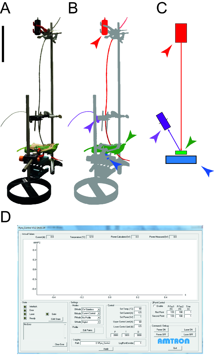
Figure 1: Apparatus used to determine leaf thermal properties. A. Photograph of the measurement apparatus used to determine the specific heat capacity and thermal conductivity of leaves. The peripheral devices (computers, oscilloscope) are not shown. B. Schematic representation of the measurement apparatus. The laser and connected equipment are highlighted in red, the NIR detector for temperature measurement is shown in purple, the leaf sample is green and the photodiode power sensor is blue. C. Drawing of the elements of the measurement setup with the same color code as in B. The size bar indicates 0.1 m. D. Screenshot illustrating the typical elements of the laser control software. Please click here to view a larger version of this figure.

Protocol

1. Plant Cultivation and Sample Preparation

1. Flush each mineral wool block with 1-2 L of deionized water and subsequently with 1 L of 0.1% [m/v] fertilizer solution. Place one tobacco (Nicotiana tabacum or N. benthamiana) seed in each block and gently flush with 0.25 L of fertilizer solution without washing away the seed.
2. Cultivate the plants for 7 weeks in a greenhouse or phytotron with 70% relative humidity, a 16-h photoperiod (180 µmol s⁻¹ m⁻²; λ = 400-700 nm) and a 25/22 °C light/dark temperature regime.
3. Move the plants to the measurement apparatus. If the plants are immobile, harvest single leaves for the measurement of thermal properties.

2. Determine Leaf Thickness and Density

1. Determine the leaf thickness
   1. Prepare a 2% [m/v] agarose solution in phosphate-buffered saline (PBS) and autoclave it. Let the solution cool down to 40 °C and embed a leaf sample placed in a Petri dish. Solidify the agarose by placing the Petri dish in a refrigerator at 4 °C for 30 min.
   2. Cut the agarose block into 200-µm slices using a vibratome with a razor blade cutting angle of 15°. Use a cutting velocity of 1.0 mm s^-1 and an amplitude of 0.5 mm.
   3. Mount five transversal leaf sections on a glass slide using cyanoacrylate as a fixative. Determine the leaf thickness under a microscope with a 20× objective and an eyepiece with 10× magnification, using the measurement tools built into the microscope software according to the manufacturer's instructions.
   4. Determine the leaf thicknesses in sample areas without veins.
   5. Alternatively, determine the leaf thickness with a dial-gauge at a vein-free area of the leaf blade. Make sure the dial-gauge is held perpendicular to the plane of the leaf blade.
      CAUTION: Cyanocrylate is a skin irritant and may also glue fingers together if not handled with care.
2. Determine the leaf density
   1. Determine the empty mass (m₀) of a dry pycnometer, then fill it with water and determine the mass again (m₁). Dry the pycnometer completely, place a leaf inside and determine the mass (m₂) once more. With the leaf inside, carefully fill up the pycnometer with water and determine the mass (m₃).
   2. Calculate the leaf density (_Ps) using Equation 1.
      Equation 1:

3. Determine the Spectral Transmission and Reflection of Leaves

1. Place a leaf in the sample chamber of a UV/VIS spectrophotometer by fixing it between sample-holding clamps. For transmission measurements, place the leaf in front of the detector. For reflection measurements place the leaf at the rear of the detection chamber.
2. Launch the spectrophotometer control software. Select a spectrum from 900 nm to 1600 nm. Start a new scan and record the values for transmission (µ_T) and reflection (µ_R) displayed by the UV/VIS spectrophotometer software, based on the spectral curve.
3. Perform all measurements with at least three biological replicates. Increase the number of biological replicates to five or more if a heterogeneous sample quality can be expected, i.e., variation in leaf surface morphology and thickness.
4. Calculate the power for transmission (P_T) and reflection (P_R) by multiplying the measured µ_T or µ_R values by the measured laser power P_Laser according to Equations 2 and 3.
   Equation 2:
   Equation 3:
   NOTE: The transmission can be also determined with a photodiode sensor during the measurement (see 6.3).

4. Set up the Measurement Apparatus

1. Mount a fiber-coupled single-bar NIR diode laser (wavelength = 1,550 nm) into a 25.4-mm diameter cone on a stainless-steel holder. Connect a controller to set the output power (P_Laser) of the NIR laser to 4-6 W.
2. Place a bi-convex lens with a focal length of 25.4 mm at the end of the cone to adjust the beam width to 13 mm.
3. Place a photodiode power sensor 354 mm below the bottom of the lens. Then attenuate the photodiode by placing a neutral density filter with an optical density of 1.0 and a 22-mm ceramic layer above the sensor.
4. Connect the photodiode power sensor to an oscilloscope using a coaxial cable.
5. Connect a 10 × 10 cm frame which has a 6 × 6 cm sample exposure area with the scaffold of the measurement setup at a height of 308 mm below the lens (Figure 1). Fix the leaf position in space by mounting it into the 10 × 10 cm frame.
6. Connect a NIR detector to a personal computer using a universal serial bus (USB) cable and install the interface software for the detector.
7. Place the detector at a 45° angle to the laser beam 135 mm above the ceramic layer. Align the measurement area of the detector to the laser spot on the sample by varying the sensor position and angle until the maximum temperature signal is observed.
8. Use the laser control interface software to adjust the output laser power to 5 W and the duration of the laser pulse to 0.5 s. Select the "Current control" command in the control options window below the graphical representation of the laser power and adjust the laser power by typing "5" into the "Power [W]" field. Adjust the laser pulse duration by typing "0.5" into the "Time [s]" field.
9. To determine the absolute laser power for each set of experiments, replace the photodiode power sensor with a thermal surface absorber power sensor at the end of each set of experiments and measure the laser output power for 20 s without a sample.

5. Prepare the Leaf Samples

1. Use intact and undamaged leaves for the measurements.
2. If relevant for the investigation, mimic typical leaf damage types by piercing the leaf with a scalpel, rubbing the leaf between latex gloves, exposing the leaf to an open flame or a laser beam for 2-3 s, or use other techniques to simulate other types of damage.
3. Carefully but quickly mount the leaf sample between sample-holding clamps.

6. Take the Temperature Measurements

1. Avoid direct contact between the leaf and the ceramic attenuator placed above the photodiode sensor to prevent artificial heat transfer that interferes with the calculation of c_p,s and λ (see section 9).
2. Use the temperature measurement software to collect the temperature profile of the leaf sample for a total of 60 s via the NIR detector. First, record the temperature baseline for 10 s, then activate the laser for 0.5 s and continue data collection for 49.5 s.
   1. Start a measurement by clicking "Measurement" and then "New Measurement". Afterwards click the green arrow above the graphical representation of the thermal profile. Save the temperature profile by clicking on the "Save" icon (a stylized disk) above the graphical representation of the profile.
3. Confirm the transmitted laser power using the photodiode power sensor by calculating the difference in signal for measurements with and without a leaf sample using an oscilloscope connected to the photodiode power sensor via a coaxial cable (Figure 2).
   1. Determine the height of the two flanks (f_1,S and f_2,S) in the voltage profile acquired with the oscilloscope.
   2. Repeat the measurement without a leaf sample as a reference (f_1,0 and f_2,0). Calculate transmission µ_T as the ratio of these measurements according to Equation 4 (see also Figure 2).
      Equation 4: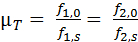

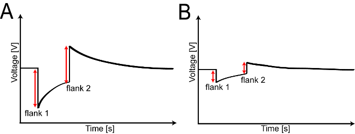
Figure 2: Measuring leaf transmission using a photodiode power sensor. A. Typical voltage profile for a reference experiment without a leaf sample visualized using an oscilloscope. B. Voltage profile with a leaf sample mounted in the apparatus. In both cases, the transmitted laser power is proportional to each of the two flanks. Please click here to view a larger version of this figure.

7. Calculate the Specific Heat Capacity of the Leaf Sample

1. Calculate the maximum temperature difference ΔT [K] during the laser pulse by subtracting the room temperature T₀ [K] from the maximum leaf temperature T_max [K] (Equation 5).
   Equation 5:
2. Calculate the energy absorbed by a leaf (E_S [J]) based on the effective laser power and laser pulse duration (Equation 6), where P_R [W] is the reflected laser power and P_T [W] is the transmitted laser power.
   Equation 6:
3. Calculate the mass of the heated leaf area (m_S [kg]) using Equation 7, where d_S [m] is the leaf thickness according to 2.1), r_Laser [m] is the radius of the laser spot, V_S [m³] is the heated leaf volume, and ρ_S [kg m^-3] is the leaf density according to 2.2).
   Equation 7:
4. Calculate c_p,s[J kg^-1 K^-1] according to Equation 8 by dividing the absorbed energy E_S by the product of the heated leaf area mass m_S and maximum temperature difference ΔT.
   Equation 8:

8. Prepare the Temperature Profile Data for Thermal Conductivity Calculations

1. Use the "Export" command of the NIR sensor control software to export the time and temperature raw data as a *.dat file and open the file in a spreadsheet processor.
2. Apply 1:100 data reduction, e.g., using an "IF(MOD(Value;100)=0;"x";"0")" command, resulting in a data density of one data point per 0.1 s.
3. Calculate the average baseline temperature T_B [°C] for each temperature profile over the initial 10 s of a measurement, during which the laser was still off. Then, calculate the difference between T_B and the actual ambient temperature T₀ [°C].
4. Use this difference to individually normalize each profile by shifting it towards T₀ (y-normalization), e.g., if T_B-T₀ = 2.0 K, then subtract 2.0 K from each temperature value in the temperature profile (Figure 3A).
5. Normalize the time coordinate of each temperature profile (x-normalization) by deleting every data point before the maximum sample temperature (T_max) and assign new time values starting with t = 0 for T_max (Figure 3B).
6. Screen each profile for sudden temperature shifts, i.e., temperature differences that are more than three times the baseline noise level, which is typically 3 × 0.31 K ≈ 1.0 K. Remove these regions from the data set because they correspond to measurement artifacts (Figure 3C).
7. Fit an exponential decay function (Equation 9) to the data using a spreadsheet processor, where T_t [K] is the fitted leaf sample temperature at time t [s], T₀ is the ambient temperature, A [K] is the amplitude and t₁ [s] the decay constant (Figure 3D).
   Equation 9: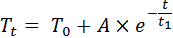
8. Use the fitted function to calculate the temperature decline in the leaf sample from 0-80 s after the laser pulse.
9. Transform the temperature data measured in [°C] to the [K] scale by adding a value of 273.15 to each temperature data point (Figure 3E).

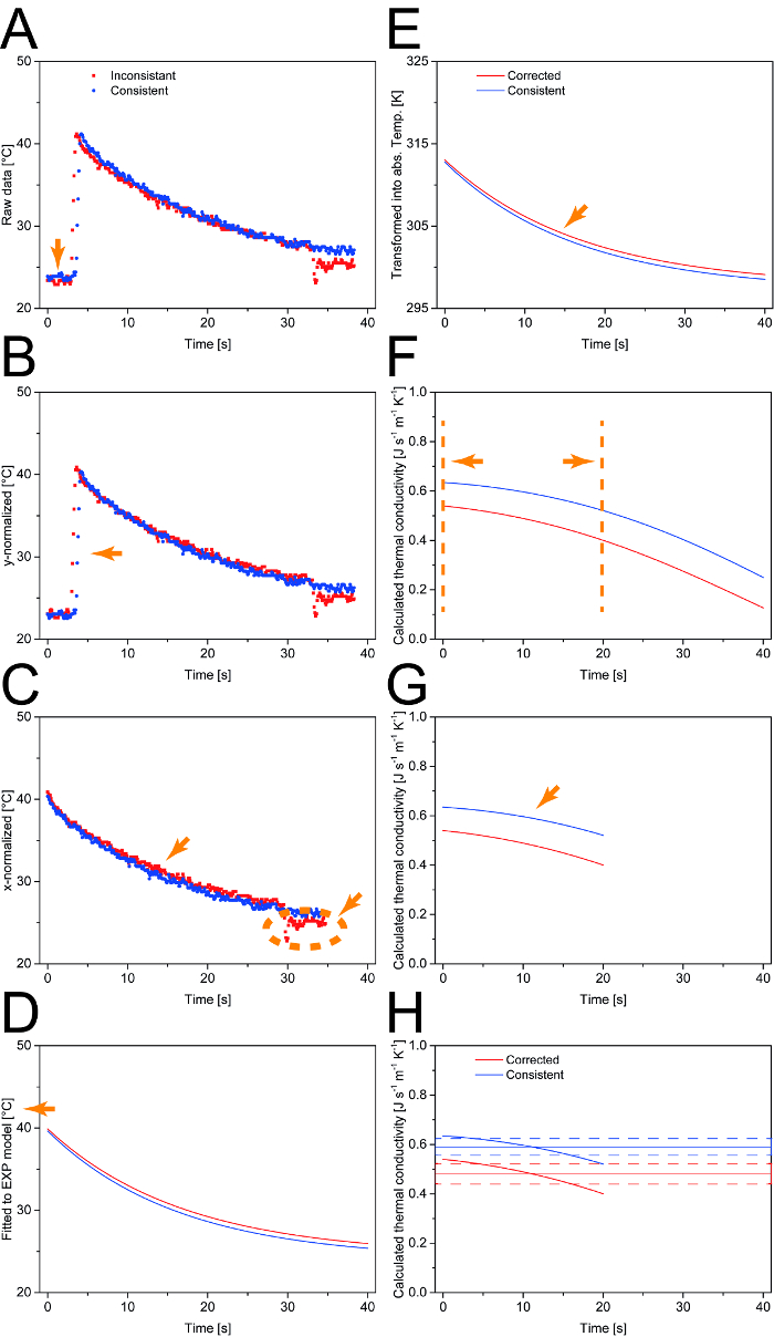
Figure 3: Data processing scheme for the calculation of λ. A. After data reduction, the temperature profiles are normalized to the ambient temperature. B. Next, all data points before the maximum sample temperature (T_max) are removed. C. Measurement artifacts (shown in the "inconsistent" data set) are identified based on temperature shifts larger than three times the baseline noise and removed from the dataset prior to fitting to an exponential function. D. The Celsius temperature scale is converted into the Kelvin scale. E. For each time interval, λ is calculated based on the temperature profile. F. A window of 20 s is defined in which a relevant temperature change can be observed. G. Based on the selected time window, the average and standard deviation are calculated for λ. H. Representative results for two different N. tabacum leaf samples. Orange arrows and lines indicate the effect of the corresponding processing step on the presented data. Please click here to view a larger version of this figure.

9. Calculation of the Thermal Conductivity of the Leaf Sample

1. Calculate the temperature difference between the leaf sample and the environment for each 0.1-s interval according to Equation 10, where ΔT_x [K] is the temperature difference, T_t [°C] is the fitted leaf sample temperature and T₀ [°C] the ambient temperature (Figure 3E).
   Equation 10: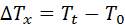
2. Assume that the decline in temperature is due to the combined effect of convective heat transfer, thermal radiation and thermal conduction. Use the corresponding energy balance (Equation 11) as a basis for the calculation of λ, where ΔE_Temp[J] is the difference in the thermal energy of the sample at two consecutive time points, ΔE_rad [J] is the energy difference due to thermal radiation, ΔE_conv [J] is the energy difference due to convective heat transfer, and ΔE_cond [J] is the energy difference due to thermal conduction.
   Equation 11:
3. Substitute the general terms in the energy balance with the actual physical properties yielding Equation 12, where ΔT_t [K] is the difference in the fitted leaf sample temperature, ε the unitless emissivity, σ [kg s^-3 K^-4] the Stefan-Boltzmann constant, A_rad [m²] the area of thermal radiation, h [J s^-1 m^-2 K^-1] the convective heat transfer coefficient, A_conv [m²] the area of convective heat transfer, A_cond [m²] the area of thermal conduction and l [m] the characteristic length.
   Equation 12:
   
4. Calculate the characteristic length l based on the correlation: l = V/A.
5. Use the heated sample volume V_S and the cross-sectional area of the leaf sample to calculate A [m²]. The cross-sectional leaf area corresponds to A_cond according to Equation 13, where A_cond is the area where conduction occurs, r_Laser is the radius of the laser spot and d_s is the leaf thickness.
   Equation 13:
6. Calculate A_rad and A_conv according to Equation 14, where A_Laser is the area of the laser spot.
   Equation 14:
7. Substitute Equations 9, 12 and 13 into Equation 11 and resolve the latter for λ, yielding Equation 15 where t_Laser is the laser pulse duration [s].
   Equation 15:
   
8. Assume a value of 0.94 for ε and calculate λ for each 0.1-s time interval over the first 20 s of the temperature profile. Average the 200 values for λ obtained in this way and calculate the standard deviation (Figure 3F − H).

Results

Measurement of Leaf Properties

Using the above microscopic method, a leaf thickness of 0.22-0.29 × 10⁻³ m was determined for both N. tabacum (0.25±0.04 × 10⁻³ m, n=33) and N. benthamiana (0.26±0.02 × 10⁻³ m, n=24), which is well within the 0.20-0.33 × 10⁻³ m range previously reported for the leaves of variou...

Discussion

The contact-free, non-destructive measurement method described above can be used to determine c_p,s and ʎ in a simultaneous and reproducible manner. The calculation of ʎ in particular depends on several parameters that are sensitive to errors. Nevertheless, the impact of these errors was either linear or sub-proportional, and the coefficient of variation for all parameters was found to be less than 10%. Even though the method can thus be regarded as robust, some technical improvements can be ...

Materials

List of materials used in this article

Name	Company	Catalog Number	Comments
1" tube	Thorlabs	SM1L10E	Tube for fiber holder
Agarose	Sigma Aldrich	A0701	Agarose
Bi-Convex lense f=25.4	Thorlabs	LB1761	Lense
Digital Handheld Optical Power and Energy Meter Console	Thorlabs	PM100D	Console for thermal surface absorber sensor
Digital Phosphor Oscilloscope	Tektronix	DPO7104	Oscilloscope
DMR light microscope	Leica	n.a.	Light microscope
Falcon 50 mL Conical Centrifuge Tubes	Fisher Scientific	14-432-2	Pycnometer
Ferty 2 Mega	Kammlott	5.220072	Fertilizer
Fiber holder	Thorlabs		Fiber holder
Forma -86 °C ULT freezer	ThermoFisher	88400	Freezer
Greenhouse	n.a.	n.a.	For plant cultivation
Grodan Rockwool Cubes 10 x 10 cm	Grodan	102446	Rockwool block
Infrared Detector Optris CT	Optris	OPTCTLT15	Infrared detector
Infrared Detector Software Compact Connect	Optris	n.a.	Control software for infrared detector
Lambda 1050 UV/Vis spectrophotometer	PerkinElmer	L1050	UV/VIS Spectrophotometer
Laser 400 μm, 1,550 nm Conduction Cooled Single Bar Fiber Coupled Module	DILAS	M1F-SS2.1	Laser
Laser cover	Amtron	LM200	Laser Cover
Laser Driver	Amtron	CS 408	Laser Driver
Osram cool white 36 W	Osram	4930440	Light source
Photodiode sensor	Thorlabs	PDA20H-EC	Power sensor for transmission measurements
Precision weight Ohaus Analytical Plus	Ohaus	80251552	Precision weight
Sample frame	Fraunhofer ILT	n.a.	Fixation of the leaf sample
Software Pyro Control	Amtron	n.a.	Laser Power Control Software
Stainless-steel-holder	n.a.	n.a.	Holder for measurement set-up
Teflon plates 2 cm	Fraunhofer ILT	n.a.	Teflon attenuation
Thermal surface absorber Power sensor	Thorlabs	S314C	Sensor for laser power measurements
Vibratome	Leica	1491200S001	Vibratome
Zoc/Pro 6.51	EmTec Innovative Software	n.a.	Laser Control Software

References

- Wilhelm, E. Heat Capacities: Liquids, Solutions and Vapours. , Royal Society of Chemistry. 516(2010).
- Costa, J. M., Grant, O. M., Chaves, M. M. Thermography to explore plant-environment interactions. J. Exp. Bot. 64, 3937-3949 (2013).
- Jayalakshmy, M. S., Philip, J. Thermophysical Properties of Plant Leaves and Their Influence on the Environment Temperature. International Journal of Thermophysics. 31, 2295-2304 (2010).
- Buyel, J. F. Process development strategies in plant molecular farming. Curr. Pharm. Biotechnol. 16, 966-982 (2015).
- Schuster, A. C., et al. Effectiveness of cuticular transpiration barriers in a desert plant at controlling water loss at high temperatures. AoB PLANTS. 8, (2016).
- Parker, W. J., Jenkins, R. J., Abbott, G. L., Butler, C. P. Flash Method of Determining Thermal Diffusivity, Heat Capacity, and Thermal Conductivity. J Appl Phys. 32, 1679-1684 (1961).
- Hays, R. L. The thermal conductivity of leaves. Planta. 125, 281-287 (1975).
- Menzel, S., et al. Optimized blanching reduces the host cell protein content and substantially enhances the recovery and stability of two plant derived malaria vaccine candidates. Front. Plant Sci. , (2015).
- Buyel, J. F., Hubbuch, J., Fischer, R. Blanching intact leaves or heat precipitation in an agitated vessel or heat exchanger removes host cell proteins from tobacco extracts. J. Vis. Exp. , Under review (2015).
- Beiss, V., et al. Heat-precipitation allows the efficient purification of a functional plant-derived malaria transmission-blocking vaccine candidate fusion protein. Biotechnol. Bioeng. 112, 1297-1305 (2015).
- Buyel, J. F., Gruchow, H. M., Tödter, N., Wehner, M. Determination of the thermal properties of leaves by non-invasive contact free laser probing. J. Biotechnol. 217, 100-108 (2016).
- Buyel, J. F. Numeric simulation can be used to predict heat transfer during the blanching of leaves and intact. Biochem. Eng. J. , (2015).
- Hedlund, H., Johansson, P. Heat capacity of birch determined by calorimetry: implications for the state of water in plants. Thermochim Acta. 349, 79-88 (2000).
- Chandrakanthi, M., Mehrotra, A. K., Hettiaratchi, J. P. A. Thermal conductivity of leaf compost used in biofilters: An experimental and theoretical investigation. Environ. Pollut. 136, 167-174 (2005).
- Larcher, W. Physiological Plant Ecology: Ecophysiology and Stress Physiology of Functional Groups. , Springer Science & Business Media. (2003).
- Cowen, R. A gamma-ray burst's enduring fireball. Science News. 152, 197(1997).
- Jones, H. G., et al. Thermal infrared imaging of crop canopies for the remote diagnosis and quantification of plant responses to water stress in the field. Funct. Plant Biol. 36, 978-989 (2009).
- Defraeye, T., Verboven, P., Ho, Q. T., Nicolai, B. Convective heat and mass exchange predictions at leaf surfaces: Applications, methods and perspectives. Comput. Electron. Agric. 96, 180-201 (2013).
- Arndt, S. K., Irawan, A., Sanders, G. J. Apoplastic water fraction and rehydration techniques introduce significant errors in measurements of relative water content and osmotic potential in plant leaves. Physiol. Plant. 155, 355-368 (2015).
- Jones, H. G., Schofield, P. Thermal and other remote sensing of plant stress. General and Applied Plant Physiology. 34, 19-32 (2008).
- Jones, H. G., Archer, N., Rotenberg, E., Casa, R. Radiation measurement for plant ecophysiology. J. Exp. Bot. 54, 879-889 (2003).
- Dupont, C., Chiriac, R., Gauthier, G., Toche, F. Heat capacity measurements of various biomass types and pyrolysis residues. Fuel. 115, 644-651 (2014).
- Chaerle, L., et al. Multi-sensor plant imaging: Towards the development of a stress-catalogue. Biotechnol. J. 4, 1152-1167 (2009).
- Hackl, H., Baresel, J. P., Mistele, B., Hu, Y., Schmidhalter, U. A Comparison of Plant Temperatures as Measured by Thermal Imaging and Infrared Thermometry. J. Agron. Crop. Sci. , 415-429 (2012).
- Yuan, L., et al. Spectral analysis of winter wheat leaves for detection and differentiation of diseases and insects. Field Crops Res. 156, 199-207 (2014).
Access restricted. Please log in or start a trial to view this content.
Reprints and Permissions