Electrophysiological Analysis of human Pluripotent Stem Cell-derived Cardiomyocytes (hPSC-CMs) Using Multi-electrode Arrays (MEAs)

Summary

Electrophysiological characterization of cardiomyocytes derived from human Pluripotent Stem Cells (hPSC-CMs) is crucial for cardiac disease modeling and for determining drug responses. This protocol provides the necessary information to dissociate and plate hPSC-CMs on multi-electrode arrays, measure their field potential, and a method for analyzing QT and RR intervals.

Abstract

Cardiomyocytes can now be derived with high efficiency from both human embryonic and human induced-Pluripotent Stem Cells (hPSC). hPSC-derived cardiomyocytes (hPSC-CMs) are increasingly recognized as having great value for modeling cardiovascular diseases in humans, especially arrhythmia syndromes. They have also demonstrated relevance as in vitro systems for predicting drug responses, which makes them potentially useful for drug-screening and discovery, safety pharmacology and perhaps eventually for personalized medicine. This would be facilitated by deriving hPSC-CMs from patients or susceptible individuals as hiPSCs. For all applications, however, precise measurement and analysis of hPSC-CM electrical properties are essential for identifying changes due to cardiac ion channel mutations and/or drugs that target ion channels and can cause sudden cardiac death. Compared with manual patch-clamp, multi-electrode array (MEA) devices offer the advantage of allowing medium- to high-throughput recordings. This protocol describes how to dissociate 2D cell cultures of hPSC-CMs to small aggregates and single cells and plate them on MEAs to record their spontaneous electrical activity as field potential. Methods for analyzing the recorded data to extract specific parameters, such as the QT and the RR intervals, are also described here. Changes in these parameters would be expected in hPSC-CMs carrying mutations responsible for cardiac arrhythmias and following addition of specific drugs, allowing detection of those that carry a cardiotoxic risk.

Introduction

Human Pluripotent Stem Cells (hPSCs) have the capacity to self-renew and generate virtually any cell type of the human body through differentiation^1,2. Detailed protocols on how to direct differentiation of hPSCs into several cardiac lineages (ventricular, atrial, pacemaker-like cardiomyocytes) have been described^3,4,5,6,7. Cardiomyocytes are electrically active cells and detailed knowledge of their electrophysiological activity can be extremely informative for understanding heart development and disease⁸. Patient-specific hiPSC-derived cardiomyocytes (hiPSC-CMs) have been successfully used to model and study the cellular, molecular, and electrical features of several cardiac arrhythmias, including Long QT Syndrome (LQTS)^{9,10,11,12,13}, Brugada syndrome¹⁴, and cathecolaminergic polymorphic ventricular tachycardia^15,16. Furthermore, multiple drugs have been added to diseased hiPSC-CMs to recapitulate therapeutic intervention and to rescue the cellular pathological phenotypes^{10,15,20,21,22}. More recently, screening platforms based on WT hiPSC-CMs have been developed, in response to the need for human systems to the early phases of drug discovery^23,24,25 as rodent cardiomyocytes differ profoundly from humans in ion channel expression and biophysics²⁶.

For this purpose, technologies suitable for medium- to high-throughput application are being developed and implemented. These include optical recordings of membrane potential, Ca²⁺ transients and strain, impedance measurements (as an indirect measure of cell contractility), and extracellular field potential (FP) measurements (for review see reference²⁴). Multi-electrode Arrays (MEA) devices allow recording of the electrical waveform signals (or FPs) generated and shaped by monolayers or small clusters of cardiomyocytes. FP contour correlates with the cardiac action potential and, to some extent, with the electrocardiogram (ECG) recordings²⁷; they typically show an initial rapid upstroke corresponding to the Na⁺ influx and membrane depolarization (R/Q peak), a slow wave/plateau phase likely corresponding to the Ca²⁺ influx, and a repolarization phase corresponding to a predominant K⁺ efflux (T peak). Perturbation of the FP waveform can be correlated with changes in specific action potential phases²⁸.

Although patch clamp recordings of action potentials could be more informative, especially for parameters as upstroke velocity and resting membrane potential, manual measurements are not feasible for experiments at medium- and high-throughput scale, while automated patch clamp has only recently been applied to hPSC-CMs²⁹. However, since prolonged recordings on MEAs allow both acute and chronic exposure to compounds to be studied, it is now possible to use hPSC-CM platforms for drug screening, discovery^24,30 and for safety pharmacology^31,32. This holds the promise of future precision or personalized medicine³³.

The purpose of this protocol is to provide the necessary information for dissociating and plating hPSC-CMs on MEA chips and measuring their FP. In this procedure, each step has been optimized, ensuring optimal cell survival and recovery after dissociation, optimal cell attachment to the MEA plate and standardized analysis and quantification of parameters. In particular, the procedure for extracellular FP recording, analysis of QT and RR intervals, and evaluation of drug effects are explained and exemplified.

Protocol

1. Preparation of Solutions and Reagents

1. Prepare hPSC-CM culture medium using low-insulin, bovine serum albumin, polyvinylalcohol, essential lipids (LI-BPEL) medium^34,35,36 by combining the reagents described in Table 1. Filter the medium through a 0.22 µm pore filter and store at 4 °C for up to 2 weeks.
2. Prepare human recombinant fibronectin stock solution by reconstituting 1 mg of human recombinant fibronectin in 5 mL of sterile distilled water to reach 200 µg/mL concentration, aliquot, and store at -80 °C.
3. Prepare 1% (w/v) enzyme detergent solution (see Table of Materials), to help removal of residual cells from the microarray chip, by dissolving 1 g of enzyme detergent powder in 100 mL of warm (~40-45 °C) deionized water. Allow the solution to cool down and store at 4 °C for up to one year.

2. Sterilization of MEA Chips (Figure 1A)

NOTE: Several different configurations of the MEAs are available, with single- or multi-well formats. The protocol described here uses the single chamber MEA containing 60 recording electrodes in an 8 x 8 grid arrangement (see Table of Materials). The electrode diameter is 30 µm and the distance between electrodes is 200 µm. One reference electrode is also present.

1. Rinse the chip thoroughly with deionized water.
2. Put the MEA chips inside a glass Petri dish that can be autoclaved. Wrap the dish in aluminum foil.
3. Sterilize the chips in a laboratory pressure cooker for 6 min. Allow the dishes to cool down before opening.
   NOTE: Alternatively, the chips can be sterilized by immersing them in 1 mL of 80% (v/v) ethanol at RT for 15-30 min.
4. Place the chips in a cell culture hood and expose the surface to UV light for approximately 30 min.

3. Coating of MEA Chips (Figure 1B and 1C)

1. Place the clean chips inside a standard 10 cm Ø plastic sterile Petri dish.
2. Add 8 mL sterile distilled water to the Petri dish to form a humidified chamber, which will prevent the small volume of culture medium on the chip to dry when placed in the incubator.
3. Use custom-made polytetrafluoroethylene (PTFE) rings (Figure 1B) to ensure plating of the cardiomyocytes in the center of the chip, where the electrode array is located. (The PTFE rings are previously stored in 80% ethanol.) In the culture hood, remove the rings from the ethanol, place them in a sterile Petri dish without a lid and allow the rings to dry in the hood.
4. Place a dry ring inside one MEA chip using flame-sterilized tweezers (Figure 1C).
   NOTE: Alternatively use 80% ethanol to wash the tweezers and allow to dry in the tissue-culture hood before using them.
5. Thaw one aliquot of human recombinant fibronectin stock (200 µg/mL in distilled water) and dilute in PBS with Ca²⁺ and Mg²⁺ to obtain a working solution of 40 µg/mL. Coat the electrodes by adding 50 µL of 40 µg/mL fibronectin inside the ring.
   NOTE: Coating using human recombinant fibronectin ensures optimal hPSC-CM attachment. However, other types of coating proteins such as bovine fibronectin or extracellular matrix proteins mixtures can be used.
6. Close the lid of the 10 cm Ø plastic Petri dish and carefully transfer the dish containing the MEA chip into the incubator. Incubate at 37 °C for at least 1 h, or at 4 °C O/N.
7. Transfer the dish containing the MEA chip to the cell-culture hood. Before using the MEA chip, aspirate the 50 µL of fibronectin using a P200 pipette or a vacuum system in the hood, without displacing the PTFE ring. Use plastic tips for this step. Ensure that no solid objects (e.g., pipette tips) touch the inside of the dish as this can damage the electrodes.
   NOTE: This will extend the life of MEA chips.
8. Gently add 950 µL of LI-BPEL medium (see Table 1 and Table of Materials), ensuring that it is evenly distributed and that the ring does not float. Return the dish to the incubator.

4. hPSC-CMs Dissociation and Plating (Figure 2)

NOTE: The protocol here described makes use of hPSC-CMs that were differentiated in a monolayer culture using cytokines³⁴ at ~18 days after starting the differentiation. However, it has been proven to be suitable for any 2D and 3D hPSC-CM culture. When using differentiated cultures at earlier or later time points, adjusting the incubation time of the dissociation enzyme (see Table of Materials) might be necessary. The following volumes are meant for a single well of a 12-well plate format (3.8 cm²).

1. Aspirate the medium from the hPSC-CMs culture well.
2. While working under a tissue culture hood, add 1-2 mL/well of PBS without Ca²⁺/Mg²⁺ to wash the culture. Aspirate the PBS.
3. Add 500 µL/well of the dissociation enzyme. Incubate for 5 min at 37 °C.
4. Add 1 mL LI-BPEL/well to dilute the enzyme. Gently detach the monolayer of hPSC-CMs by gently scratching using a P1000 pipette. Collect the cell suspension in a 15 mL tube.
5. Rinse the well with 1 mL LI-BPEL to collect all the remaining cells and cell clumps.
6. Add another 2-3 mL of LI-BPEL to reach a final volume of 5-6 mL and gently pipette up and down 3-5x with a 5 mL pipette to dissociate cell clumps.
   NOTE: Dissociation into single cells at this point is not necessary, since it will affect cell survival. Presence of small clusters will ensure higher cell viability.
7. Centrifuge the cells at RT for 3 min at 300 x g.
8. Remove the supernatant, trying to remove most of the surplus fluid but without dislodging the cell pellet.
9. Resuspend the cell pellet in 250 µL LI-BPEL (using a P1000 and pipetting extremely gently).
10. Distribute ~50 µL of cell suspension per MEA (up to 5 MEAs can be prepared from one well of a 12-well plate) by pipetting the cell suspension directly into the center of the PTFE ring, on top of the electrode array.
    NOTE: At this stage cells are difficult to count due to the presence of cell clusters and the total number of cells per MEA can substantially vary, depending on the hPSC-CM source used. While plating, ensure that the cloud of dissociated cells covers the area of the electrodes.
11. Carefully transfer the MEAs to the incubator at 37 °C and allow the cells to attach O/N

5. Ring Removal and Medium Refreshment (Figure 3)

1. At 1 day after plating, carefully remove the ring in a sterile environment using sterile tweezers (Figure 3A-3B).
2. Rinse the ring in 80% (v/v) ethanol and store it in a 50 mL tube containing fresh 80% (v/v) ethanol.
3. Gently remove 500 µL of medium from the MEA chip and add 500 µL of fresh LI-BPEL.
4. Transfer the MEAs to the incubator at 37 °C.
   NOTE: The cells should start beating 1-7 days after ring removal and medium change (Figure 3C).
5. Measure electrical activity of hPSC-CMs on MEAs 1-7 days after ring removal.

6. Check Signal Quality (Figure 4)

1. Switch on the computer and launch the software suite linked to the MEA set up: TCX-Control, MC_MEA Select and MC_Rack. Set the temperature to 37 °C in TCX-Control to record measurements at physiological temperature.
2. Remove the dish containing the MEA chip from the incubator. Open the lid, take out the MEA chip, and place it on a tissue to absorb residual water.
3. Carefully wipe the external contacts of the plate with a tissue and clean them using a cotton swab moistened with 100% (v/v) ethanol to remove any residual water or debris, which might cause signal noise.
4. Transfer the MEA plate to the heated (37 °C) recording head-stage to detect the spontaneous activity (e.g., hardware: see Table of Materials; software: MC_Rack).
   1. Open MC_Rack: Click 'Edit' → 'Add MC_Card' to create a new protocol. Use the drop down menu 'Edit' to add different Recorder and Display windows to the protocol.
      NOTE: A sampling frequency of at least 10 kHz is recommended. The protocol we use contains one Longterm Display Tool, with a full layout of the whole MEA chip, and one Spike Sorter, essential to capture drug effect in real time. The Spike Cutout is tuned with a 'Pre Trigger' of 20 ms, a 'Post Trigger' of 800 ms and a 'Dead Time' of 2 ms. The protocol can be saved as '.rck' file and reloaded before starting the experiments.
5. Start the protocol in play mode by clicking on the 'play' button.
   NOTE: At this point it is possible to reload the protocol saved under step 6.5. In MC_Rack, load the protocol (.rck file extension) by clicking 'File' → 'Open'.
6. If the signals exhibit clearly visible R peaks and T peaks, wait 10-15 min to conclude the adaptation phase. Examples of good and bad quality traces are shown in Figure 4.
   NOTE: If no T-peak can be detected in any of the electrodes, do not proceed with the experiment. Usually this is the result of poor electrical activity of the hPSC-CMs or poor attachment of the cells to the electrodes.

7. Start Experiment and Recording

1. Click 'record' and then 'play', and acquire data for 10 min under baseline conditions to determine the steady state. Annotate the electrodes that have the best signal so that they can be easily identified and exported later for the analysis.
2. For drug-response assessment, add increasing concentrations of drug at every 10 min. As an example, add the hERG blocker E4031 at a final concentration of 1 μM. For this, remove 100 μL of medium and add the same volume of 10 μM E4031 dissolved in the medium.
   NOTE: As previously demonstrated by Cavero and colleagues³¹, a wise choice of the volume in which the drugs are dissolved is important, since it can profoundly alter the drug response curve.
3. Repeat step 7.2 for all the other drug concentrations of interest.
4. Click 'stop' to conclude the recordings at the end of the protocol.

8. MEA Cleaning for Reuse

1. Once the experiment recording is finished, gently remove the medium with a P1000 pipette. Do not to touch the inside of the dish as this can damage the electrodes. Discard according to local safety rules.
2. Rinse the MEA chips with deionized water using a wash bottle, and repeat the wash step 3-4x.
   NOTE: At this point it is not necessary that the cells are completely detached from the chip.
3. Add 1 mL of enzyme detergent solution 1% (v/v) into each well and incubate O/N at 4 °C to allow cell detachment and cell removal.
4. One day later, rinse the MEA chips thoroughly with deionized water to remove enzyme detergent solution and residual cells and add 1 mL deionized water. Clean MEA chips can be stored immersed in deionized water at 4 °C.

9. Data Export

1. Open the MC_Data Tool software linked to the MEA set up.
2. Click 'File' → 'Open MCD'.
3. Click 'Tools' → 'Convert MCD to ABF'.
4. Select the electrodes with the best recording signals to be exported for the analysis. Choose the directory in which to save the exported files and click 'Save'. The export procedure may take several min depending on the number of the electrodes exported and the total size of the recording files.

10. Data Analysis

1. Download and install an electrophysiology data acquisition and analysis program (e.g., pClamp). Once complete, launch the analysis software (e.g., Clampfit).
2. RR Interval calculation (Figure 5).
   1. Place two vertical cursors to define the region of interest on the trace. Select 'Event detection' → 'Threshold Search'. The horizontal cursor should cross all the events that must be quantified, as shown in Figure 5A.
   2. Click 'OK' and then 'Accept the Entire Category'. The software will then search through the trace for all the suitable events. Blue marks will be placed above the events.
   3. Adjust the sensitivity of the automatic selection by tuning the parameters in the main event detection window.
   4. Once all the events have been automatically identified, go to the result window (Window → Results) and copy the column entitled "Intervent Interval", which contains the frequency data (Figure 5B).
3. QT Interval calculation (Figures 6-9):
   1. Place one cursor right before and one after a single FP at the steady state condition. Select 'Event Detection' → 'Create Template' (Figure 6).
   2. Check that the FP is correctly identified and click 'Add'. The template will be moved to the bottom panel.
   3. Save the template as a '.atf' file. In this way, a template trace has been created that will be searched by the software throughout the entire recording (Figure 7). Create one template for each condition, since a drug effect might alter the shape of the FP. If necessary, filter the trace slightly to include a maximum of 10.000 points within the two cursors.
   4. Once the template has been saved with '.atf' extension, select 'Event Detection' → 'Template Search' and load the template.
   5. Adjust the "Template match threshold" to correctly identify all the FP in the selected interval.
   6. Once all the events have been correctly identified, save them in a new '.abf' file.
4. Open the file with analysis software and automatically calculate the 'Time of Peak' for both the Q/R and the T peaks (Figures 8, 9). If traces are very noisy, apply a filter. Calculate the QT interval by subtracting the Q/R value from the T value in a spreadsheet editor of choice.

Results

One day after dissociation and plating, the layer of hPSC-CMs will be visible as a dense and white film covering the center of the MEA chamber (Figure 3A). After removal of the ring (Figure 3B), the layer should remain in place and inspection on a light microscope will show the MEA electrodes covered by the (contracting) hPSC-CM layer (Figure 3C). Because of physical and electrical coupling of the cells, only one electrode (golden electrode) will be used for analysis.

Alternatively, when working with 3D structures, such as embryoid bodies or microtissues, these can be plated so that they are physically and electrically uncoupled. Visual inspection at the microscope could confirm no physical connection between the clusters and nonsynchronized R waves at MEAs confirm no electrical coupling. In this case, multiple independent electrodes can be analyzed.

Typical recordings of FP traces are shown in Figure 4. In particular, a good quality trace can be defined by the presence of a clear peak corresponding to the Na⁺ influx and membrane depolarization (R/Q peak), a clear repolarization phase corresponding to K⁺ efflux (T peak), and a high signal to noise ratio (Figure 4A, left: note y-axis scale and Figure 4B). Bad quality traces (Figure 4A, middle) may be the result of failure of hPSC-CMs to attach to the MEA plate or of weak hPSC-CM electrical activity. Waiting 1-3 days for better attachment may improve the signal; however, if no signal improvement is visible, excluding this MEA from experiments is recommended. Noisy traces (Figure 4A, right) may be analyzed after filtering.

Successful analysis of RR interval can be identified by visual inspection of the screen showing peak detection (Figure 5A, 5B). Within the time interval defined by the vertical cursors, blue marks corresponding to each peak should be present. In case the program does not identify one or more peaks, try to move the horizontal cursor and run the analysis again or adjust the detection settings. Similarly, successful analysis of QT interval can be identified by visual inspection of the screen showing FP detection (Figure 7). Within the time interval defined by the vertical cursors, blue marks corresponding to each FP detection should be present. In case the program does not identify one or more FPs, try to redefine the FP template (Figure 6) or adjust the detection settings and run the analysis again.

Extracted individual FP traces or their average (Figure 8) can be used for obtaining QT interval values with specific settings as in Figure 9. Analysis of QT-RR relationship is advisable and is meaningful in diseased and WT hPSC lines (Figure 10A) and to evaluate the need and/or the effect of QT-interval corrections (Figure 10B-10D). hPSC-CMs carrying LQTS-causing mutations have prolonged QT intervals compared with WT controls (Figure 11A). Treatment of hPSC-CMs with a hERG blocker results in QT interval prolongation (Figure 11B); conversely, treatment with a hERG activator results in shortening of the QT interval (Figure 11C). Finally, treatment with drugs affecting the beating frequency of hPSC-CMs should be visible as a change in the RR interval (Figure 11D, RR interval shortening).

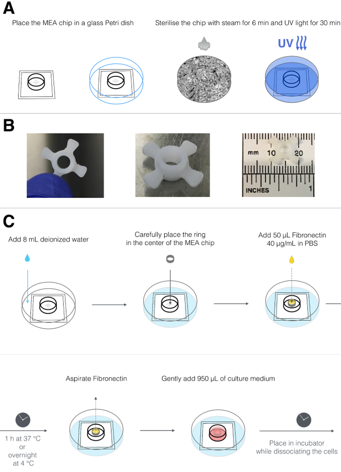
Figure 1: Sterilization and Coating of MEA Chips. (A) Scheme representing the sterilization process including placing the MEA chip in an autoclavable glass Petri dish, wrapping up in aluminum foil, steaming for 6 min, and exposing to UV for 30 min. (B) Top (left panel) and side (middle panel) views of custom PTFE ring; the ring has an outer diameter of 1.2 cm, including 4 flaps that allow its positioning in the center of the MEA chip and the inner diameter is 0.4 cm (right panel). (C) Schematic representing preparation of the MEA chip including placing the chip in a standard plastic Petri dish, adding 8 mL of deionized water outside the MEA chamber, placing the PTFE ring in the middle of the chamber, and coating the electrode array with fibronectin. After incubation time, fibronectin is removed and replaced with culture medium. Please click here to view a larger version of this figure.

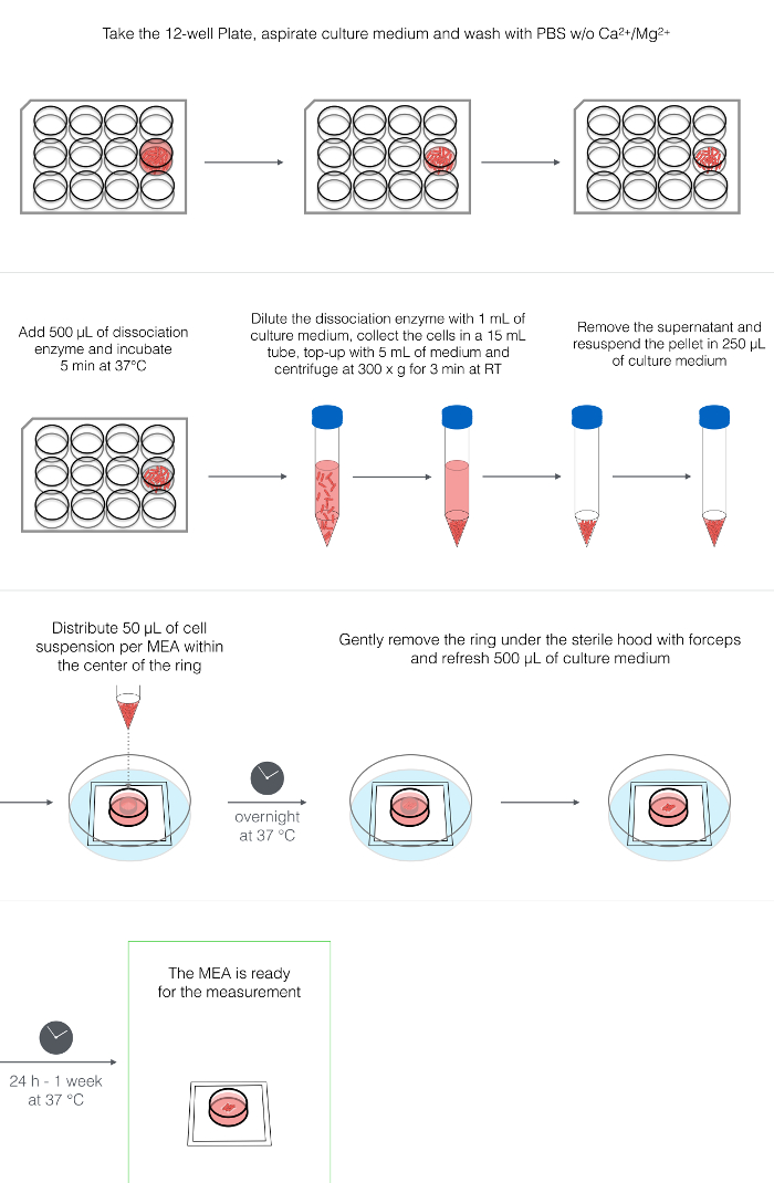
Figure 2: Dissociation and Plating of hPSC-CMs. Schematic representing the processes of hPSC-CMs enzymatic dissociation, centrifugation, resuspension, and plating on the center of the MEA chamber. Please click here to view a larger version of this figure.

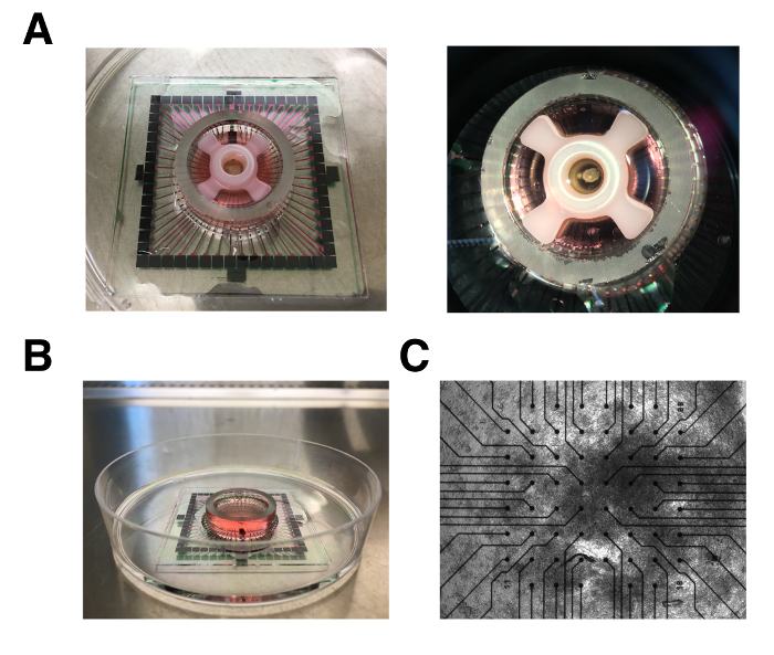
Figure 3: MEA Chips with hPSC-CM Layer. (A) Top views of MEA chip containing the ring and the layer of hPSC-CMs. (B) side view of MEA chip after ring removal. (C) Bright field image of hPSC-CMs layer plated on the micro-electrode array; 4X magnification. Please click here to view a larger version of this figure.

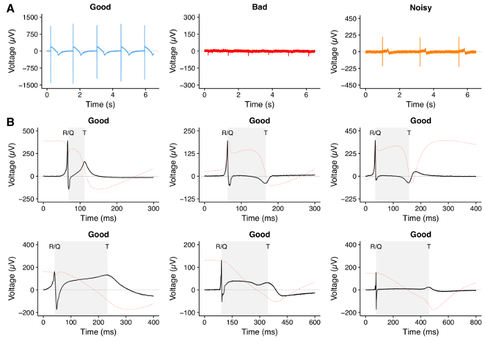
Figure 4: MEA Recording of hPSC-CMs. (A) Representative traces recorded with the MEA showing a good quality trace with R/Q and T peaks clearly visible with high signal to noise ratio (left), a bad quality trace without clearly visible R/Q and T peaks (middle), and a noisy trace with R/Q and T peaks clearly visible but with low signal to noise ratio (right). (B) Representative examples of good quality FP traces with different morphologies that can be recorded during MEA experiments using hPSC-CMs. The shaded area represents the QT interval measured during the analysis. Since the FP at MEA resembles the first derivative of the action potential²⁸, we have calculated the integral of the FP trace, shown as red dotted line, as theoretical demonstration of a T wave choice close to a complete action potential repolarization. Please click here to view a larger version of this figure.

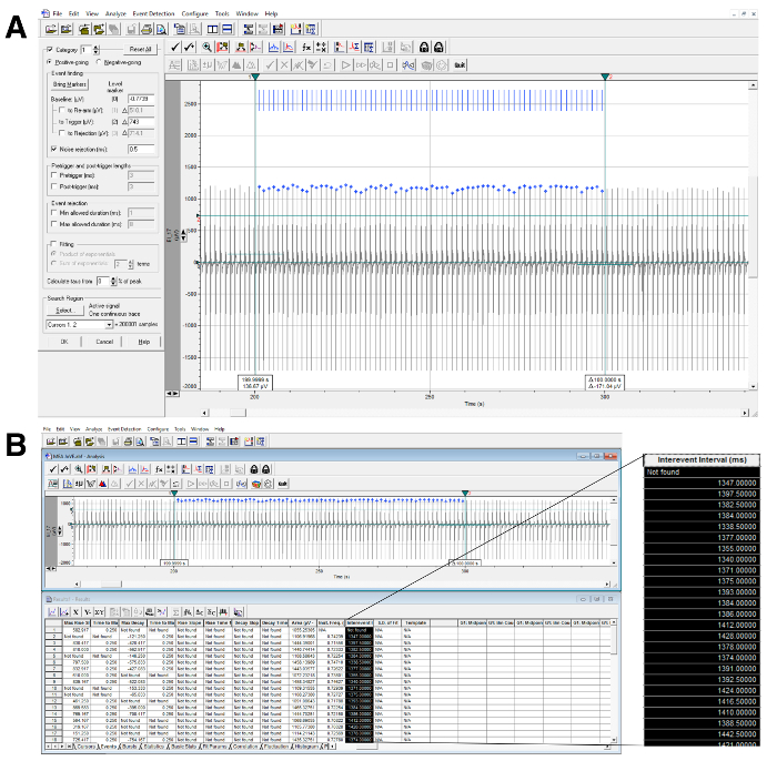
Figure 5: RR Interval Calculation. (A) Example of RR interval analysis with automatic peak detection (top) and data extraction (bottom) using the analysis software (see Table of Materials). Vertical cursors identify the time interval of interest and the horizontal cursor is crossing all the events that are detected and identified by blue marks. (B) The magnified column shows the extracted data used to calculate the RR interval. Please click here to view a larger version of this figure.

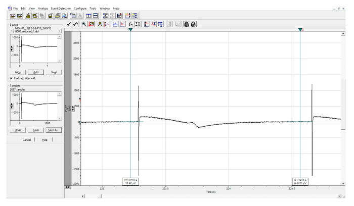
Figure 6: Creation of FP Template. Example of template selection using vertical cursors placed before and after a single FP. This template is used for FP automatic identification. Please click here to view a larger version of this figure.

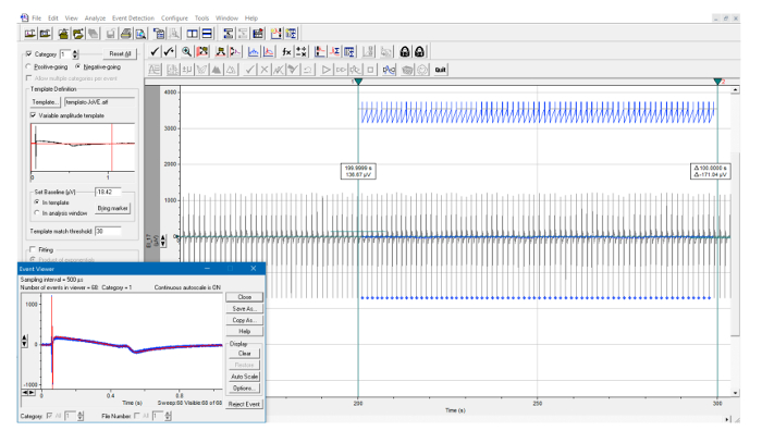
Figure 7: FP Template Automatic Identification. Example of template search throughout an interval defined by two vertical cursors. All the detected events are identified by blue marks and are automatically superimposed in the inset. Please click here to view a larger version of this figure.

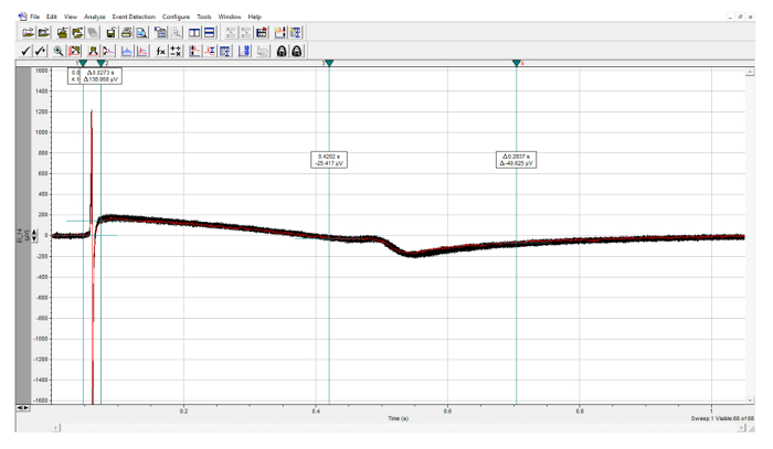
Figure 8: Quantification of FP Parameters. Analysis of the saved events, with the R peak manually identified within the first two cursors and the T peak manually identified within the last two cursors. Please click here to view a larger version of this figure.

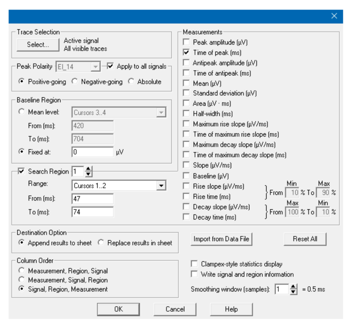
Figure 9: Analysis Window. Parameters used in the Statistics window to detect R peak. For the detection of the T peak, change cursors and (if necessary) polarity. Please click here to view a larger version of this figure.

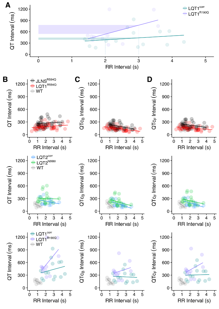
Figure 10: QT-RR Relationship. (A) Example of different relationship between QT and RR intervals between WT (LQT1^corr) and Long QT syndrome type 1 (LQT1^R190Q) hPSC-CMs. Shaded areas show that the same shift in RR interval generates a bigger shift in the QT interval of the LQT1 diseased line, thus likely increasing arrhythmia susceptibility. (B) Relationship between uncorrected QT and RR intervals measured at MEA in CMs from 7 different hPSC lines. The effect of QT correction for Bazett's (C) or Fridericia's (D) formulae is shown and visible as change in the slope of the QT-RR interval relationship. Figures adapted from reference³⁰. Please click here to view a larger version of this figure.

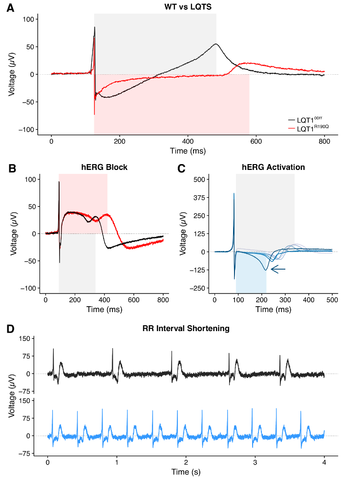
Figure 11: Disease- or Drug-induced QT and RR Interval Variations. (A) Example of QT interval prolongation in hPSC-CM derived from a patient carrying a Long-QT Syndrome (LQTS) mutation compared to its isogenic WT control. (B) Example of QT interval prolongation in hPSC-CM upon pharmacological hERG block. (C) QT interval shortening upon treatment with increasing doses of hERG activator. Arrow indicates the direction of the shortening. (D) Example of drug-induced RR interval shortening. Panel (C) was adapted from reference³⁰. Please click here to view a larger version of this figure.

Low-insulin, BSA, polyvinylalcohol, essential lipids (LI-BPEL) Medium
Component		Quantity for 100 mL
IMDM		43 mL
F12		43 mL
Ascorbic Acid 2-phosphate (5 mg/mL in distilled water)		1 mL
Cell culture supplement (direct substitute for L-glutamine)		1 mL
Penicillin/Streptomycin		0.5 mL
Phenol Red		1 mg
Protein Free Hybridoma Medium-II (PFHMII)		5 mL
BSA (10% wt/vol in IMDM)		2.5 mL
PVA (5% wt/vol in distilled water)		2.5 mL
Chemically Defined Lipid Concentrate (CDLC)		1 mL
Insulin-Transferrin-Selenium-Ethanolamine (ITS-X) 100X		0.1 mL
α-Monothioglycerol (13 µL in 1 mL IMDM)		0.3 mL
Combine the reagents, filter with a 0.22 µm pore filter and store the medium at 4 °C for up to 2 weeks.

Table 1: Li-BPEL Medium Composition.

Discussion

This protocol shows how to dissociate and prepare hPSC-CMs for measuring their FP using MEAs. hPSC-CMs usually display spontaneous electrical activity, which can be measured as FP and can provide meaningful data with respect to beating frequency, QT interval duration, and arrhythmic events.

Dissociation of 2D cardiac differentiated cultures is needed for recreating a beating layer on the MEA and it represents a critical step. Mechanical stress by repeated pipetting and/or aggressive dissociation enzyme treatments may result in high cell mortality, failure to attach to the MEA plate, and lack of spontaneous electrical activity. This protocol has been optimized for monolayer cultures. However, a similar approach can be used for three-dimensional (3D) cultures (e.g., embryoid bodies or EBs) with minor modifications, such as collection of the EBs followed by PBS wash and longer incubation time with the dissociating enzyme. Importantly, in both 2D and 3D differentiated cultures, the older the differentiated cells, the longer incubation time required might be to detach the cells because of increased extracellular matrix deposition.

The protocol described here for quantifying FP parameters can be used to generate dose-response curves for cardioactive drugs. As recently described by Cavero et al.³¹, the starting concentration of a drug might profoundly affect the outcome of a MEA measurement. Therefore, to improve accuracy and reliability of the results, we suggest the following: 1) in case of irreversible activators/blockers, use relatively large volumes of medium containing the drug to be tested. More in detail, remove 10-50% of medium volume from the MEA chip and add an equal volume of medium in which the drug was previously dissolved at the appropriate concentration. In this case, for calculating the final drug concentration, it is critical to consider the change in concentration after medium removal. 2) In case of reversible activators/blockers, add 10 µL of each drug dose from a 100X stock solution.

The majority of the cardiac differentiation protocols results in a variable mixed population of nodal-like, atrial-like and ventricular-like cardiomyocytes, with the ventricular type being the most represented. This might constitute a limitation when modeling cardiac diseases affecting a specific cardiomyocyte subtype or drugs acting on cardiac subtype-specific ion channels. Although several studies have optimized conditions to direct more controlled specification during cardiac differentiation^3,5,37,38, their broader applicability is still under investigation.

Furthermore, variable efficiency of differentiation (in different experiments and in different hPSC lines) might be observed^{39,40,41,42,43,44}. Cardiomyocyte-enriching strategies based on surface protein expression^35,45 (by florescence-assisted cell sorting or by magnetic-bead selection^46,47), and metabolic selection^44,48 may represent valid strategies that can be applied to any (genetically modified or unmodified) hPSC-line prior plating of the hPSC-CMs, to improve the electrical signal.

Although hPSC-CMs are notoriously immature as compared to human adult cardiomyocytes^4,49, they have proven to be valuable in recapitulating and identifying specific disease-related changes (e.g., in channelopathies)^19,20,50 and drug-induced responses (e.g., cardiac ion channel blockers)^4,51. Furthermore, immature cells are easier to dissociate, and recover better than adult cardiomyocytes after dissociation and plating⁴⁴ therefore, hPSC-CM immaturity may be rewarded as an advantage in this respect. However, to be able to recapitulate e.g. late onset cardiac diseases and faithfully reproduce drug responses of adult cardiomyocytes, a more mature mechanical, metabolic, and electrical hPSC-CM state should be obtained. Methods to mature these cells include prolonged time in culture⁵², mechanical strain⁵³, electrical pacing⁵⁴, addition of small molecules⁵⁵, 3D-culture⁵⁶, co-culture with other cell types⁵⁷, and even a combination of these approaches⁵⁸; to date, none of these approaches has led to an adult-like phenotype.

As part of the immaturity features, hPSC-CMs show electrical automaticity. Here, details are provided on how to accurately quantify QT and RR intervals. One limitation of measuring spontaneous electrical activity is that comparison of QT intervals may be difficult when hPSC-CMs display different beating frequencies. In this case, Bazett's or Fridericia's formulae can be used to correct the QT interval for the frequency. However, as previously reported³⁰, we strongly recommend performing Major-Axis regression analysis by plotting QT interval versus RR interval for both raw and corrected data, to exclude any possible bias due to the correction method itself.

The protocol presented here, together with previously described methods^59,60 helps the standardization of the procedures and the analysis of hPSC-CM FPs, improving data reproducibility and allowing a better comparison of inter-laboratory results.

Materials

List of materials used in this article

Name	Company	Catalog Number	Comments
Biological safety cabinet/laminar flow-hood	Cleanair
MEA2100 in vitro recording system	Multi Channel Systems
CO2 cell-culture incubator	Sanyo	MCO-15A
Centrifuge	Hitachi	himac-CT6EL
Leica stereomicroscope	Leica Microsystems	MS5
Handheld pipetman (P-10 (10 μL), P-200 (200 μL), P-1000 (1,000 μL))	Gilson International
Filter tips (10 μL, 200μL, 1,000μL)	Corning	4807 (10 μL), 4810 (200μL), 4809 (1000μL)
Disposable bottle top filter (0.22 μm pore size)	Millipore	SCGVU02RE
Sterile plastic pipette	Greiner Bio-One	606180 (5 mL), 607180 (10 mL), 760180 (25 mL)
Tweezers	Dumont
Autoclavable Petri dishes	VWR/ Duran Group	391-0860
MEA chip	Multi Channel Systems	MEA200/30iR-Ti-gr
Phosphate-buffered Saline (PBS) calcium, magnesium	Thermo Fisher Scientific	14040-091
Phosphate-Buffered Saline (PBS) no calcium, no magnesium	Thermo Fisher Scientific	14190-169
Human recombinant fibronectin	Tebu-Bio	J64560
Custom-made polytetrafluoroethylene (PTFE) MEA rings	LUMC: department of Instrument Development
Dissociation enzyme - TrypLE Select 1x	Thermo Fisher Scientific	12563-029
Tergazyme enzyme detergent	Sigma-Aldrich	Z273287-1EA
Distilled Water	Thermo Fisher Scientific	15230-089
Name	Company	Catalog Number	Comments
Reagents for LI-BPEL medium
Iscove's Modified Dulbecco's Medium (IMDM)	Thermo Fisher Scientific	21056-023
F12 nutrient mixture (Ham)	Thermo Fisher Scientific	31765-027
Ascorbic Acid 2-phosphate	Sigma-Aldrich	A8960
Glutamax	Thermo Fisher Scientific	35050-038
Penicillin/Streptomycin	Thermo Fisher Scientific	15070-063
Phenol Red	Sigma-Aldrich	P3532
Protein-free Hybridoma Medium-II (PFHMII)	Thermo Fisher Scientific	12040-077
Bovine Serum Albumin (BSA)	Bovogen Biologicals Australia	BSAS05
Poly(Vinyl Alcohol) (PVA)	Sigma-Aldrich	P8136
Chemically-defined Lipid Concentrate (CDLC)	Thermo Fisher Scientific	11905-031
Insulin-Transferrin-Selenium-Ethanolamine (ITS-X) 100x	Thermo Fisher Scientific	51599-056
α-Monothioglycerol	Sigma-Aldrich	M6145
Name	Company	Software version	Comments
MC_Rack	Multi Channel Systems	4.6.2	Alternatively, data can be recorded using Cardio2D or MC_Experimenter (MultiChannel Systems)
TCX Control	Multi Channel Systems	1.3.4
MEA Select	Multi Channel Systems	1.3.0
MC_Data Tool	Multi Channel Systems	2.6.15	Alternatively, Multi Channel Data Manager (MultiChannel Systems) can be used when custom data export is required (HDF5, EDF, etc.)
Clampfit	Molecular Devices	7.0.0	Used in step 10.1 for analyzing, graphing, and formatting of all of data. To use Clampfit, download and install the electrophysiology data acquisition and pClam (latest version, 10.7.0), available on the Molecular Devices Website. Once complete, launch the software Clampfit. Alternatively, data can be analysed using Cardio2D (MultiChannel Systems) or MatLab custom code.

References

- Takahashi, K., et al. Induction of pluripotent stem cells from adult human fibroblasts by defined factors. Cell. 131 (5), 861-872 (2007).
- Thomson, J. A., et al. Embryonic stem cell lines derived from human blastocysts. Science. 282 (5391), 1145-1147 (1998).
- Birket, M. J., et al. Expansion and patterning of cardiovascular progenitors derived from human pluripotent stem cells. Nat Biotechnol. 33 (9), 970-979 (2015).
- Denning, C., et al. Cardiomyocytes from human pluripotent stem cells: From laboratory curiosity to industrial biomedical platform. Biochim Biophys Acta. 1863 (7 Pt B), 1728-1748 (2016).
- Devalla, H. D., et al. Atrial-like cardiomyocytes from human pluripotent stem cells are a robust preclinical model for assessing atrial-selective pharmacology. EMBO Mol Med. 7 (4), 394-410 (2015).
- Lewandowski, J., Kolanowski, T. J., Kurpisz, M. Techniques for the induction of human pluripotent stem cell differentiation towards cardiomyocytes. J Tissue Eng Regen Med. , (2016).
- Mummery, C. L., Zhang, J., Ng, E. S., Elliott, D. A., Elefanty, A. G., Kamp, T. J. Differentiation of human embryonic stem cells and induced pluripotent stem cells to cardiomyocytes: a methods overview. Circ Res. 111 (3), 344-358 (2012).
- Davies, M. P., An, R. H., Doevendans, P., Kubalak, S., Chien, K. R., Kass, R. S. Developmental changes in ionic channel activity in the embryonic murine heart. Circ Res. 78 (1), 15-25 (1996).
- Bellin, M., et al. Isogenic human pluripotent stem cell pairs reveal the role of a KCNH2 mutation in long-QT syndrome. EMBO J. 32 (24), 3161-3175 (2013).
- Moretti, A., et al. Patient-specific induced pluripotent stem-cell models for long-QT syndrome. N Engl J Med. 363 (15), 1397-1409 (2010).
- Ma, D., et al. Modeling type 3 long QT syndrome with cardiomyocytes derived from patient-specific induced pluripotent stem cells. Int J Cardiol. 168 (6), 5277-5286 (2013).
- Yazawa, M., et al. Using induced pluripotent stem cells to investigate cardiac phenotypes in Timothy syndrome. Nature. 471 (7337), 230-U120 (2011).
- Limpitikul, W. B., et al. A Precision Medicine Approach to the Rescue of Function on Malignant Calmodulinopathic Long QT Syndrome. Circ Res. , (2016).
- Liang, P., et al. Patient-Specific and Genome-Edited Induced Pluripotent Stem Cell-Derived Cardiomyocytes Elucidate Single-Cell Phenotype of Brugada Syndrome. J Am Coll Cardiol. 68 (19), 2086-2096 (2016).
- Jung, C. B., et al. Dantrolene rescues arrhythmogenic RYR2 defect in a patient-specific stem cell model of catecholaminergic polymorphic ventricular tachycardia. EMBO Mol Med. 4 (3), 180-191 (2012).
- Novak, A., et al. Cardiomyocytes generated from CPVTD307H patients are arrhythmogenic in response to beta-adrenergic stimulation. J Cell Mol Med. 16 (3), 468-482 (2012).
- Bellin, M., Mummery, C. L. Inherited heart disease - what can we expect from the second decade of human iPS cell research. FEBS Lett. 590 (15), 2482-2493 (2016).
- Sallam, K., Li, Y., Sager, P. T., Houser, S. R., Wu, J. C. Finding the rhythm of sudden cardiac death: new opportunities using induced pluripotent stem cell-derived cardiomyocytes. Circ Res. 116 (12), 1989-2004 (2015).
- Sinnecker, D., Goedel, A., Laugwitz, K. L., Moretti, A. Induced pluripotent stem cell-derived cardiomyocytes: a versatile tool for arrhythmia research. Circ Res. 112 (6), 961-968 (2013).
- Bellin, M., Marchetto, M. C., Gage, F. H., Mummery, C. L. Induced pluripotent stem cells: the new patient? Nat Rev Mol Cell Biol. 13 (11), 713-726 (2012).
- Sinnecker, D., Laugwitz, K. L., Moretti, A. Induced pluripotent stem cell-derived cardiomyocytes for drug development and toxicity testing. Pharmacol Ther. 143 (2), 246-252 (2014).
- Terrenoire, C., et al. Induced pluripotent stem cells used to reveal drug actions in a long QT syndrome family with complex genetics. J Gen Physiol. 141 (1), 61-72 (2013).
- Abi-Gerges, N., et al. Assessment of extracellular field potential and Ca2+ transient signals for early QT/pro-arrhythmia detection using human induced pluripotent stem cell-derived cardiomyocytes. J Pharmacol Toxicol Methods. 83, 1-15 (2016).
- Del Alamo, J. C., et al. High throughput physiological screening of iPSC-derived cardiomyocytes for drug development. Biochim Biophys Acta. 1863 (7 Pt B), 1717-1727 (2016).
- Blinova, K., et al. Comprehensive Translational Assessment of Human Induced Pluripotent Stem Cell Derived Cardiomyocytes for Evaluating Drug-Induced Arrhythmias. Toxicol Sci. , (2016).
- Nerbonne, J. M. Studying cardiac arrhythmias in the mouse--a reasonable model for probing mechanisms? Trends Cardiovasc Med. 14 (3), 83-93 (2004).
- Halbach, M., Egert, U., Hescheler, J., Banach, K. Estimation of action potential changes from field potential recordings in multicellular mouse cardiac myocyte cultures. Cell Physiol Biochem. 13 (5), 271-284 (2003).
- Tertoolen, L. G., Braam, S. R., van Meer, B. J., Passier, R., Mummery, C. L. Interpretation of field potentials measured on a multi electrode array in pharmacological toxicity screening on primary and human pluripotent stem cell-derived cardiomyocytes. Biochem Biophys Res Commun. , (2017).
- Rajamohan, D., et al. Automated Electrophysiological and Pharmacological Evaluation of Human Pluripotent Stem Cell-Derived Cardiomyocytes. Stem Cells Dev. 25 (6), 439-452 (2016).
- Sala, L., et al. A new hERG allosteric modulator rescues genetic and drug-induced long-QT syndrome phenotypes in cardiomyocytes from isogenic pairs of patient induced pluripotent stem cells. EMBO Mol Med. 8 (9), 1065-1081 (2016).
- Cavero, I., Guillon, J. M., Ballet, V., Clements, M., Gerbeau, J. F., Holzgrefe, H. Comprehensive in vitro Proarrhythmia Assay (CiPA): Pending issues for successful validation and implementation. J Pharmacol Toxicol Methods. , (2016).
- Sala, L., Bellin, M., Mummery, C. L. Integrating cardiomyocytes from human pluripotent stem cells in safety pharmacology: has the time come? Br J Pharmacol. , (2016).
- Chen, I. Y., Matsa, E., Wu, J. C. Induced pluripotent stem cells: at the heart of cardiovascular precision medicine. Nat Rev Cardiol. 13 (6), 333-349 (2016).
- Dambrot, C., et al. Strategies for rapidly mapping proviral integration sites and assessing cardiogenic potential of nascent human induced pluripotent stem cell clones. Exp Cell Res. 327 (2), 297-306 (2014).
- Elliott, D. A., et al. NKX2-5(eGFP/w) hESCs for isolation of human cardiac progenitors and cardiomyocytes. Nat Methods. 8 (12), 1037-1040 (2011).
- Ng, E. S., Davis, R., Stanley, E. G., Elefanty, A. G. A protocol describing the use of a recombinant protein-based, animal product-free medium (APEL) for human embryonic stem cell differentiation as spin embryoid bodies. Nat Protoc. 3 (5), 768-776 (2008).
- Karakikes, I., et al. Small molecule-mediated directed differentiation of human embryonic stem cells toward ventricular cardiomyocytes. Stem Cells Transl Med. 3 (1), 18-31 (2014).
- Zhang, Q., et al. Direct differentiation of atrial and ventricular myocytes from human embryonic stem cells by alternating retinoid signals. Cell Res. 21 (4), 579-587 (2011).
- Mummery, C., et al. Differentiation of human embryonic stem cells to cardiomyocytes: role of coculture with visceral endoderm-like cells. Circulation. 107 (21), 2733-2740 (2003).
- Kehat, I., et al. Human embryonic stem cells can differentiate into myocytes with structural and functional properties of cardiomyocytes. J Clin Invest. 108 (3), 407-414 (2001).
- Kattman, S. J., et al. Stage-specific optimization of activin/nodal and BMP signaling promotes cardiac differentiation of mouse and human pluripotent stem cell lines. Cell Stem Cell. 8 (2), 228-240 (2011).
- Zhang, J., et al. Extracellular matrix promotes highly efficient cardiac differentiation of human pluripotent stem cells: the matrix sandwich method. Circ Res. 111 (9), 1125-1136 (2012).
- Lian, X., et al. Directed cardiomyocyte differentiation from human pluripotent stem cells by modulating Wnt/beta-catenin signaling under fully defined conditions. Nat Protoc. 8 (1), 162-175 (2013).
- Burridge, P. W., et al. Chemically defined generation of human cardiomyocytes. Nat Methods. 11 (8), 855-860 (2014).
- Dubois, N. C., et al. SIRPA is a specific cell-surface marker for isolating cardiomyocytes derived from human pluripotent stem cells. Nat Biotechnol. 29 (11), 1011-1018 (2011).
- Fuerstenau-Sharp, M., et al. Generation of highly purified human cardiomyocytes from peripheral blood mononuclear cell-derived induced pluripotent stem cells. PLoS One. 10 (5), e0126596(2015).
- Schwach, V., Passier, R. Generation and purification of human stem cell-derived cardiomyocytes. Differentiation. 91 (4-5), 126-138 (2016).
- Tohyama, S., et al. Distinct metabolic flow enables large-scale purification of mouse and human pluripotent stem cell-derived cardiomyocytes. Cell Stem Cell. 12 (1), 127-137 (2013).
- Veerman, C. C., Kosmidis, G., Mummery, C. L., Casini, S., Verkerk, A. O., Bellin, M. Immaturity of human stem-cell-derived cardiomyocytes in culture: fatal flaw or soluble problem? Stem Cells Dev. 24 (9), 1035-1052 (2015).
- Karakikes, I., Ameen, M., Termglinchan, V., Wu, J. C. Human induced pluripotent stem cell-derived cardiomyocytes: insights into molecular, cellular, and functional phenotypes. Circ Res. 117 (1), 80-88 (2015).
- Avior, Y., Sagi, I., Benvenisty, N. Pluripotent stem cells in disease modelling and drug discovery. Nat Rev Mol Cell Biol. 17 (3), 170-182 (2016).
- Otsuji, T. G., Minami, I., Kurose, Y., Yamauchi, K., Tada, M., Nakatsuji, N. Progressive maturation in contracting cardiomyocytes derived from human embryonic stem cells: Qualitative effects on electrophysiological responses to drugs. Stem Cell Res. 4 (3), 201-213 (2010).
- Mihic, A., et al. The effect of cyclic stretch on maturation and 3D tissue formation of human embryonic stem cell-derived cardiomyocytes. Biomaterials. 35 (9), 2798-2808 (2014).
- Lieu, D. K., et al. Mechanism-based facilitated maturation of human pluripotent stem cell-derived cardiomyocytes. Circ Arrhythm Electrophysiol. 6 (1), 191-201 (2013).
- Yang, X., et al. Tri-iodo-l-thyronine promotes the maturation of human cardiomyocytes-derived from induced pluripotent stem cells. J Mol Cell Cardiol. 72, 296-304 (2014).
- Mannhardt, I., et al. Human Engineered Heart Tissue: Analysis of Contractile Force. Stem Cell Reports. , (2016).
- Kim, C., et al. Non-cardiomyocytes influence the electrophysiological maturation of human embryonic stem cell-derived cardiomyocytes during differentiation. Stem Cells Dev. 19 (6), 783-795 (2010).
- Nunes, S. S., et al. Biowire: a platform for maturation of human pluripotent stem cell-derived cardiomyocytes. Nat Methods. 10 (8), 781-787 (2013).
- Clements, M. Multielectrode Array (MEA) Assay for Profiling Electrophysiological Drug Effects in Human Stem Cell-Derived Cardiomyocytes. Curr Protoc Toxicol. 68 (22), 1-22 (2016).
- Harris, K. A Human Induced Pluripotent Stem Cell-Derived Cardiomyocyte (hiPSC-CM) Multielectrode Array Assay for Preclinical Cardiac Electrophysiology Safety Screening. Curr Protoc Pharmacol. 71, 1-15 (2015).
Reprints and Permissions