This paper describes the operation procedure for the flow tube reactor and related data collection. It shows the protocols for setting the experiments, recording data and generating the number-diameter distribution as well as the particle mass information, which gives useful information about chemical and physical properties of the organic aerosols.
Method Article
Production and Measurement of Organic Particulate Matter in a Flow Tube Reactor
In This Article
Summary
Abstract
Organic particulate matter (PM) is increasingly recognized as important to the Earth's climate system as well as public health in urban regions, and the production of synthetic PM for laboratory studies have become a widespread necessity. Herein, experimental protocols demonstrate approaches to produce aerosolized organic PM by α-pinene ozonolysis in a flow tube reactor. Methods are described for measuring the size distributions and morphology of the aerosol particles. The video demonstrates basic operations of the flow tube reactor and related instrumentation. The first part of the video shows the procedure for preparing gas-phase reactants, ozonolysis, and production of organic PM. The second part of the video shows the procedures for determining the properties of the produced particle population. The particle number-diameter distributions show different stages of particle growth, namely condensation, coagulation, or a combination of both, depending on reaction conditions. The particle morphology is characterized by an aerosol particle mass analyzer (APM) and a scanning electron microscope (SEM). The results confirm the existence of non-spherical particles that have grown from coagulation for specific reaction conditions. The experimental results also indicate that the flow tube reactor can be used to study the physical and chemical properties of organic PM for relatively high concentrations and short time frames.
Introduction
Volatile organic compounds (VOCs) emitted from the biosphere and anthropogenic activities undergo reactions in the atmosphere with oxidants (such as ozone or OH radicals) to produce secondary oxygenated compounds1,2. Some of these compounds, due to their low volatility, ultimately contribute to the mass concentration of atmospheric PM1,3,4. Atmospheric particles have important effects on climate, human health, and visibility5. The production mechanisms of organic PM, however, remain insufficiently characterized and understood, both qualitatively and quantitatively, to predict number and mass concentrations as well as physical and chemical properties. One approach for bridging this knowledge gap is to perform laboratory studies that use flow tube reactors for mimicking the production processes of atmospheric organic PM, thereby facilitating mechanistic, process, and characterization studies of the PM6,7,8,9,10,11,12. The flow tube reactor enables the rapid synthesis of aerosol particles for a variety of particle number and mass concentrations13.
The present study describes, through the use of video material, the production of organic PM as submicron-sized particles from the ozonolysis of a dominant atmospheric monoterpene (viz. α-pinene) in a flow tube reactor, which was first described in Shrestha et al.13 Briefly, the flow tube was made of glass with an inner diameter of 48.2 mm and a length of 1.30 m. The flow tube was operated slightly above ambient pressure in the laminar flow regime (Reynolds number of 9.4 ± 0.5), and with a residence time of 38 ± 1 s 14. The temperature was set to be 25 ± 1 °C by using a recirculating chiller to flow water in a double-layered customized box that housing the flow tube reactor.
A schematic plot of the flow tube reactor system is shown in Figure 1. A pure air generator is used to generate ultra-pure air that passes through an ozone generator, producing 200-500 ppm of ozone. An additional flow of pure air at 0.50 sLpm is used to evaporate α-Pinene injected by a syringe injector in a round bottom flask. α-Pinene is pre-mixed with 2-butanol at a dilution ratio of 1:5015,16,17 before being withdrawn to the syringe injector, because 2-butanol can act as an OH scavenger to ensure that ozonolysis was the only reaction occurring inside the flow tube. The round bottom flask was heated to 135 ± 1 °C allowing quick evaporation of the injected organic compounds. The α-pinene and ozone flow inlets were also arranged perpendicular to each other to induce turbulence and rapid mixing at the injection point. The outlet of the flow tube was split between sample collection, size distribution measurements (by the scanning mobility particle sizer-SMPS), particle density measurement, and exhaust. Reaction conditions are varied to control the relative contribution of condensation compared to coagulation to particle growth. The output of the flow tube needs to have at least one line connecting to an open-air exhaust hood, to ensure that it is not possible to build up pressure inside the flow tube and the round bottom flask even under incorrect experimental conditions. The characteristics of the produced particle population can thereby be finely adjusted. The flow tube reactor is equipped with a movable sampler enabling sampling of the organic PM at different time points in its production. The number-diameter distribution of the produced particle population is measured at various length of the flow tube. An APM measures the particle mass distribution and the dynamic shape factor7,18,19, which gives information about the morphology and other physical properties of the produced particle population.20,21 Particles are also collected on a nanometer particle sampler for offline imaging by an SEM7,22. The implication is that the flow tube reactor is a suitable medium for performing ozonolysis experiments and fast online and offline analysis of the PM produced therein.
Protocol
1. Gas-Phase Injection of the Flow Tube Reactor
- Organic Precursor Injection
NOTE: All the equipment and software used during the experiment can be found in the Table of Materials. Depending on the purpose of the experiments, a wide range of volatile organic compounds can be used as the organic precursor for the experiment. α-Pinene is used here as an example for the procedure of injecting the organic precursor into the flow tube reactor.- Use a micropipette to obtain 1.00 mL of α-pinene. Transfer the liquid to a 50.00 mL volumetric flask.
- Use 2-butanol to fill the volumetric flask to 50.00 mL, thereby diluting the α-pinene by a ratio of 1:50. Shake the volumetric flask to mix the solvent and the solute thoroughly.
- Use a syringe (5.00 mL) to withdraw the α-pinene solution. Rinse the syringe three times with the solution and then fill it with solution.
- Connect the syringe to a sharp needle (25 gauge, 2-inch long). Place the syringe onto a syringe injector. Insert the needle tip into a vaporizer round-bottom flask (25 mL). Pre-heat the vaporizer flask to 135 ± 1 °C by heating tape.
- Introduce a gentle flow of 0.5 sLpm purified air to vaporize and carry away α-pinene injected from the syringe. Connect the purified air generator to the same power supply as the heating tape to avoid heating the round bottom flask if the pure air supply is stopped.
- Turn on the syringe injector, and adjust the injection rate to an appropriate value. Calculate the injection rate by applying the gas flow rate, the desired VOC concentration and the syringe size to the Clausius-Clapeyron equation. For instance, for a total flow of 4.5 sLpm, to reach 125 ppb of α-pinene would require an injection rate of 11.7 μL/h of the α-pinene and 2-butanol mixture. Ensure that the volumetric concentration of butanol or α-pinene is less than 1% in the round bottom flask to avoid the organic compounds reach the flammability limit.
- Ozone Injection
- Pass a flow of air at 4.00 sLpm through an ozone generator.
- Turn on the ozone generator. Control the ozone concentration to appropriate values by adjusting the length of the glass tube shielding the UV lamp inside the generator. The ozone and VOC ratios can vary across two orders of magnitudes depending on the purpose of the experiment. If VOC is needed to be fully reacted during the experiment, then the ozone concentration should be about 10 times higher than the VOC concentration to ensure ozone is in excess.
- Turn on the ozone concentration monitor and connect the ozone monitor to the computer. Using a terminal reader software to access the ozone monitor readout and save the data obtained from the ozone monitor (Figure 2). Perform the experiments after the ozone concentration stabilizes.
2. Particle Production of the Flow Tube Reactor
- Adjustment of residence time
- Unscrew the cap at the end of the flow tube reactor to adjust the position of the movable sampler tubing inside the flow tube reactor. Change different positions of the movable sampler tubing subsequently to achieve different residence times from 3 s to 38 s10.
- During each experiment, change the position of the movable sampler to adjust the residence time of the particles being produced inside the flow tube reactor.
- Position the movable sampler at the beginning of the flow tube reactor (0.10 m from the gas inlet) to obtain the shortest residence time (3 s). Position the movable sampler at the end of the flow tube reactor (1.30 m from the gas inlet) to obtain the longest residence time (38 s).
- Temperature control for particle production
- House the flow tube reactor in a temperature-controlled, double-walled, water-jacketed stainless-steel box. Perform a leak check and a water level check prior to each set of experiments.
- Set the temperature of the thermostat in the water circulator to 20.0 °C.
NOTE: Temperature during the course of an experiment varies by no more than 0.1 °C. - Turn on the temperature recording software in the main computer, and set the data sampling time to 10 s (Figure 3). The temperature sensor is located at the center point of the flow tube. Start logging the temperature measured from the temperature sensor when turning on the Record button.
- Record the temperature for 4 to 6 h. Stabilize the temperature before performing the experiment.
NOTE: The temperature fluctuation of the flow tube reactor is less than ± 0.1 °C during a 24-hour period.
- The pressure monitoring system
- Connect a pressure monitor to the flow tube outlet through a ¼ inch connector and the main computer
- Turn on the pressure monitor software (Figure 4), and then click File | New | Time/Sample Interval to set the sampling interval to 10 s.
- Click on Total Data Points to set the sampling length to 36,000 points. Click OK to record the data.
NOTE: The outlet pressure stays within ± 0.01 atm during a 24-hour period, suggesting the pressure within the flow tube is stable.
3. Characterization of Produced Particle Population of the Flow Tube Reactor
- Number-diameter distributions
- Connect the outlet of the flow tube reactor to a scanning mobility particle sizer (SMPS) by electrostatic-resistant tubing. Similar instrument can also be used to measure the number-diameter distributions instead of the SMPS.
NOTE: The detailed operating procedures or troubleshooting of the SMPS can be found in its manual. - Start the software that records the number-diameter distribution. Create a new file by clicking on Create A New File. Set each parameter shown in Figure 5. Record the number-diameter distributions of the particles exiting the flow tube reactor by clicking on OK button.
- Connect the outlet of the flow tube reactor to a scanning mobility particle sizer (SMPS) by electrostatic-resistant tubing. Similar instrument can also be used to measure the number-diameter distributions instead of the SMPS.
- Relative humidity control
- Connect the two inlets of a water bubbler to two mass flow controllers (MFCs) so as to adjust the humidity of the sheath air in the flow tube. Adjust the flow rate of the two inlets from 0-10 sLpm so as to change the relative humidity of the sheath air from <5% to >95%.
- Connect the outlet of the water bubbler to the sheath air inlet of the permeable membrane tube. Connect the outlet of the flow tube reactor to the main sampling inlet of the same permeable membrane tube.
- Connect a relative humidity (RH) sensor to the outlet of the permeable membrane tube to measure the RH of the sampling air.
- Start the RH measuring program by clicking on the Start button, entering the file name, and clicking the Save button to record the RH data.
- Mass and dynamic shape factor of the SOM particles
- Connect the outlet of the relative humidity control setup to the inlet of a differential mobility analyzer (DMA) with a three-feet-long electrostatic-resistant tubing. Connect the outlet of the DMA to the inlet of the APM instrument by one-feet-long electrostatic-resistant tubing. Connect the outlet of the APM to a condensation particle counter (CPC).
NOTE: The detailed operating procedures or troubleshooting of the DMA and CPC can be found in its manual. - Turn on the APM instrument and the APM control box by pressing the respective power buttons. Click Remote button on the APM control box so that the instrument can be operated from the software interface in the computer.
- Turn on the APM control software. Load a pre-set scanning file by clicking the File and Load buttons (Figure 6).
- Click on the Start button of the APM control software so that the APM instrument starts to collect data.
- Connect the outlet of the relative humidity control setup to the inlet of a differential mobility analyzer (DMA) with a three-feet-long electrostatic-resistant tubing. Connect the outlet of the DMA to the inlet of the APM instrument by one-feet-long electrostatic-resistant tubing. Connect the outlet of the APM to a condensation particle counter (CPC).
- Particle collection from the flow tube reactor
- Connect the flow tube outlet to a nanometer aerosol sampler (NAS) by a three-feet-long electrostatic-resistant tubing.
- Clean a silicon substrate (prime grade, resistance 1-10 Ω∙cm) by a cycle of methanol, water, and again methanol. Dry the substrate using a gentle flow of nitrogen.
- Place the cleaned substrate onto the electrode of the NAS. Secure the edge of the substrate with tape to keep it stable during the collection22.
- Turn on the NAS. Set the voltage to -9.9 kV. Set the flow rate to 1.8 Lpm.
- Turn on the sampling instrument to run for 12-36 h. Afterwards, remove the silicon substrate loaded with collected particles from the NAS. Perform further analysis of particles on the substrate, such as morphology by SEM7 or surface analysis9.
Results
A matrix of reaction conditions is summarized in Table 1. There is a range of number and mass concentrations of organic PM that can be produced depending on the selected α-pinene and ozone concentrations13. For instance, as shown in Table 1, when the ozone concentration is 43 ppm, varying the α-pinene concentration from 0.125-100 ppm could produce (4.4 ± 0.6) × 105 to (9.1 ± 0.3) × 106 particles∙cm3 and mass concentrations of 101 to 104 µg∙m-3, respectively.
The evolution of the dynamic characteristics of the particle population can be studied inside the flow tube reactor. By means of video demonstration, an experiment was conducted using 50 ± 1 ppm of ozone and 125 ppb of α-pinene. The longitudinal position of the particle sampler inside the flow tube allowed sampling at various times from 3.0 ± 0.2 to 38 ± 1 s. Figure 7 shows the number-diameter distributions of the aerosol particle population for this experiment. The total number concentration and the mode diameter of the particles increased with the residence time. For a residence time of 3 s, no particles were detected. For longer residence times, a particle population was obtained and measured. The mode diameter increased from less than 10 nm to about 50 nm for an increase in residence time from 17 ± 0.5 s to 38 ± 1 s. The corresponding number concentration increased from (8.6 ± 0.5) × 104 cm-3 to (2.56 ± 0.07) × 105 cm3.
Examples of the number-mass distributions recorded in three replicate experiments by the APM setup are shown in Figure 8. The particle mass and mobility diameters were used to calculate the dynamic shape factor, χ, across particle subpopulation. The dynamic shape factor χ is the ratio of the drag force on an actual particle divided by the drag force experienced by a volume-equivalent sphere23. Shape factors of nearly spherical particles approach unity whereas highly aspherical particles have significantly larger shape factors. Figure 9 shows the dynamic shape factors of the particles exiting the flow tube at various mobility diameters and humidity levels. The respective χ values for <5% RH were 1.21 ± 0.02, 1.09 ± 0.02, and 1.08 ± 0.02 (one-sigma uncertainty), suggesting that the particle populations were composed largely of non-spherical particles.
As the RH was increased, χ decreased for all three populations, reaching a final value of 1.02 ± 0.01 at 35% RH and corresponding within uncertainty to spherical particles. Figure 10 shows SEM images of the particles exposed to <5% RH (left column) and 80% RH (right column). The images indicate that the non-spherical particles became round after exposure to high RH, as discussed in detail in Zhang et al.7. The results above indicate that the flow tube reactor is capable of performing various kinds of online and offline analysis.
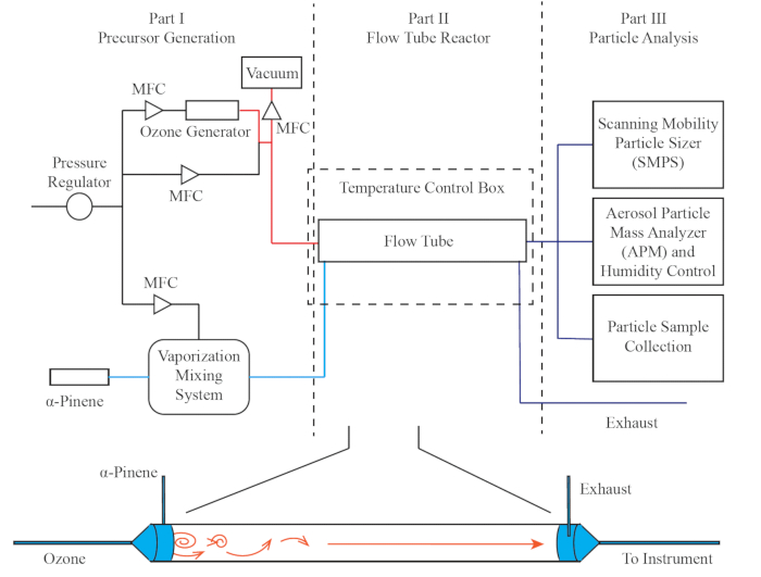
Figure 1. A schematic flow diagram of the flow tube reactor system. The red lines show the flow containing ozone, the light blue lines show the flow containing α-pinene, and the dark blue lines show the flow of the organic PM. The APM system consist of a DMA, an APM, and a CPC that are connected together. This figure previously appeared in Shreatha et al.13 and is reproduced here with permission.
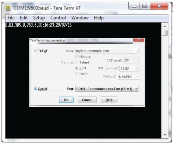
Figure 2. Graphical user interface for the ozone monitoring and recording program.
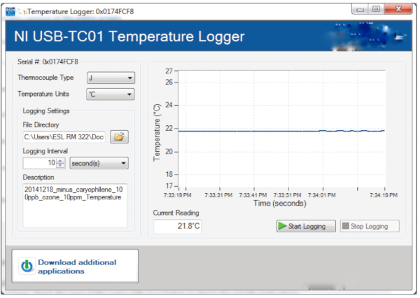
Figure 3. Graphical user interface for the temperature monitoring and recording program.
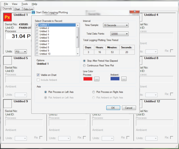
Figure 4. Graphical user interface for the pressure monitoring and recording program.
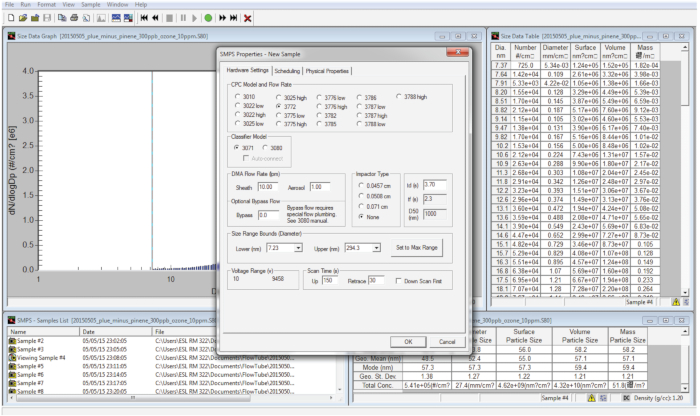
Figure 5. Graphical user interface for the number-diameter distribution program. Please click here to view a larger version of this figure.
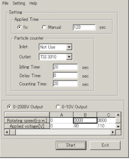
Figure 6. Graphical user interface for the APM program.
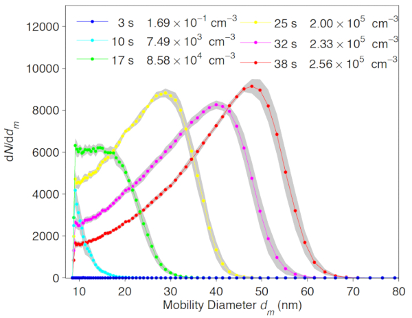
Figure 7. Size distribution of the particle population from the flow tube at different residence times. The total number concentrations for each size distribution are 1.69 × 10⁻¹, 7.50 × 10³, 8.58 × 10⁴, 2.00 × 10⁵, 2.33 × 10⁵, and 2.56 × 10⁵ particles cm-3 for residence times of 3, 10, 17, 25, 32, and 38 s, respectively. The shaded areas are the standard deviation of particle size distribution. This figure previously appeared in Shreatha et al.13 and is reproduced here with permission. Please click here to view a larger version of this figure.
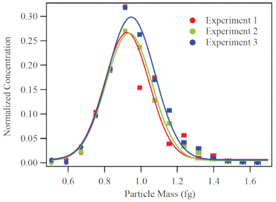
Figure 8. An example of the number-mass distribution, as measured using the DMA-APM system. Results of three replicate experiments are shown to demonstrate reproducibility. Two-sigma uncertainty is represented by the error bars, which are approximately the same size as the data markers. The lines represent fits of a normal distribution to the data. The abscissa is calculated based on the APM rotation speed and the voltage applied between the walls of the APM cylinders. The particles shown in the plot were produced from 700 ppb α-pinene and 14 ppm ozone. A central mobility diameter of 126.0 nm was selected by the DMA. This figure previously appeared in Zhang et al.7 and is reproduced here with permission. Please click here to view a larger version of this figure.

Figure 9. Dynamic shape factor for increasing relative humidity. Panel A: Particles produced from 700 ppb α-pinene and 14, 25, and 30 ppm ozone for particle populations having central mobility diameters of 126.0, 175.0, and 190.0 nm, respectively. The exposure time to relative humidity was 310 s. The error bars in each panel represent two sigma of standard deviation. This figure previously appeared in Zhang et al.7 and is reproduced here with permission. Please click here to view a larger version of this figure.
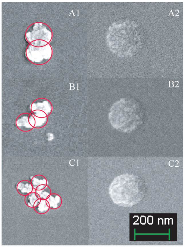
Figure 10. SEM images of the particles obtained from 700 ppb α-pinene and sampled for a central mobility diameter of 180.0 nm. The aerosol particles were collected on the silica substrate for 12 h and then coated with 5 nm of Pt/Pd. The voltage for the electron beam was 5 kV, and the working distance was 2.3 mm. Column 1 shows dimer, trimer, and higher-order agglomerates of the granular monomers for <5% RH. Red circles identify the monomers. Column 2 shows nearly spherical particles that were collected after exposure to 80% RH followed by drying to <5% RH. This figure previously appeared in Zhang et al.7 and is reproduced here with permission.
| O3 (ppm) | 0.15±0.02 | 0.9±0.1 | 5.7±0.2 | 43±1 | 194±2 | ||
| α-pinene | |||||||
| (ppm) | |||||||
| 0.125 ± 0.003 | Num. Conc. | 0 | (1±1)×102 | (1.0±0.6)×105 | (4.4±0.6)×105 | (3.2±0.2)×105 | |
| Mass. Conc. | 0 | (3±5)×10-2 | 15±5 | 11±3 | 20±2 | ||
| Mode Diameter | 0 | 22±4 | 60±5 | 35±3 | 34±2 | ||
| Geo. St. Deviation | N/A | 1.2 | 1.3 | 1.3 | 1.5 | ||
| 1.00 ± 0.03 | Num. Conc. | 0 | (3.1±0.9)×102 | (1.5±0.2)×105 | (5.5±0.2)×105 | (5.8±0.4)×105 | |
| Mass. Conc. | 0 | (9±3)×10-3 | 61±9 | (52±0.1)×102 | (66±0.1)×102 | ||
| Mode Diameter | 0 | 33±7 | 86±6 | 84±3 | 85±19 | ||
| Geo. St. Deviation | N/A | 1.3 | 1.4 | 1.5 | 1.7 | ||
| 10.0 ± 0. 3 | Num. Conc. | (2±2)×101 | (4.0±0.2)×105 | (6.0±0.7)×105 | (6.3±0.7)×105 | (1.8±0.2)×106 | |
| Mass. Conc. | 0* | (1.6±0.2)×102 | (2.5±0.2)×103 | (1.19±0.02)×104 | (1.57±0.02)×104 | ||
| Mode Diameter | 8±9 | 81±2 | 147±9 | 245±38 | 155±5 | ||
| Geo. St. Deviation | 1 | 1.4 | 1.4 | 1.4 | 1.5 | ||
| 100 ± 3 | Num. Conc. | (4.4±0.3)×105 | (8.3±0.3)×105 | (8.3±0.4)×106 | (9.1±0.2)×106 | (1.3±0.02)×107 | |
| Mass. Conc. | 35±3 | (8.6±0.1)×102 | (1.3±0.1)×104 | (1.6±0.04)×105 | (4.0±0.1)×105 | ||
| Mode Diameter | 48±2 | 88±5 | 134±8 | 262±12 | 334±4 | ||
| Geo. St. Deviation | 1.4 | 1.6 | 1.5 | 1.7 | 1.9 | ||
Table 1. Number concentrations (cm-3), mass concentrations (µg m-3), mode diameter (nm), and geometric diameter standard deviation of the particles produced by α-pinene ozonolysis. A material density of 1200 kg∙m3 was used for conversion of volume concentrations to mass concentrations and the residence time was 38 s for all experiments. *Although particles were present, the mass concentration was below the detection limit. This table previously appeared in Shreatha et al.13 and is reproduced here with permission.
Discussion
By adjusting the conditions in the flow tube reactor, a wide range of SOA particles with well-defined number concentrations and mass concentrations can be produced. The growth mechanism can also be altered between the condensational growth and coagulative growth modes, forming particles with different shapes. The critical steps in the protocol include maintaining a relative stable temperature of the flow tube reactor, and stabilizing the ozone concentration out of the ozone generator. It is also important to note that the position of the movable injector needs to be carefully recorded every time so that the residence time would stay the same when repeating the experiments.
If the particle concentration from the flow tube reactor seems to be different than expected, several troubleshooting procedures can be performed. An air-tight examine of the flow tube reactor can be performed first. Following the airtight exam, the number-diameter measurement instrument needs to be checked in order to exclude all the potential malfunction possibilities such as clogging at the inlet and depletion of 1-butanol solution for CPC.
Hence, the flow tube reactor described above is a useful tool for studying the physicochemical properties and evolution of the organic aerosols spanning a wide range of concentrations. Compared with other aerosol generation systems, the flow tube reactor can quickly produce aerosol particles for a variety of particle number and mass concentrations13, which is especially useful in high mass-loading sampling. The flow tube reactor is also equipped with a movable sampler, enabling study on the evolution and growth of the aerosol particles. On the other hand, the reactor has a relatively short residence time and a relatively high precursor concentration, which limits its ability to simulate close-to-ambient reaction conditions. Future work involving the flow tube reactor is to add ultraviolet illumination onto the inner walls so that photo-oxidation reactions can be conducted within the flow tube reactor. Plans are in place for other VOC reactants, such as β-caryophyllene and limonene, to be studied as well24.
Disclosures
The authors declare no competing financial interests.
Acknowledgements
This material is based upon work supported by the National Science Foundation Environmental Chemical Sciences Program in the Division of Chemistry under Grant No. 1111418, the Atmospheric-GeoSciences Division of the U.S. National Science Foundation (NSF) under grant number 1524731, as well as Harvard Faculty Publication Award. We acknowledge Mona Shrestha, Adam Bateman, Pengfei Liu, and Mikinori Kuwata for useful discussions and assistance with the experiments.
Materials
| Name | Company | Catalog Number | Comments |
|---|---|---|---|
| (-)-α-pinene | Sigma-Aldrich | 305715 | |
| 2-butanol | Sigma-Aldrich | 294810 | |
| 5.00 mL syringe | Hamilton | 201300 | |
| Aerosol particle mass analyzer | Kanomax | 3600 | |
| Condensational particle counter | TSI | 3022 | |
| Differential mobility analyzer | TSI | 3081 | |
| Heating mantle | Cole-parmer | WU-36225-10 | |
| Mass flow controller | MKS | M100B | |
| Nafion tube | Perma Pure | MD-700-24F-1 | |
| Nanometer aerosol sampler | TSI | 3089 | |
| Ozone generator | Jelight | 600 | |
| Ozone monitor | Ecosensors | UV-100 | |
| Pressure sensor | Omega | PX409 | |
| RH sensor | Rotronic | 60587161 | |
| Round-bottom, three neck flask | Aceglass | 6944-04 | |
| Scanning electron microscope | Zeiss | N/A | Ultra plus FESEM |
| Scanning mobility particle sizer | TSI | 3071A+3772 | electrostatic classifier is model 3071A and the condensational particle ocunter is 3772 |
| Silicon substrate | University Wafer | 1707 | |
| Syringe Needle | Hamilton | 90025 | 25 G, 2 inch |
| Syringe pump | Chemyx | Fusion Touch 200 | |
| Temperature sensor and software | National Instrument | USB-TC01 | |
| water circulator | Brinkmann | RC6 |
References
- Hallquist, M., et al. The formation, properties and impact of secondary organic aerosol: current and emerging issues. Atmospheric Chemistry and Physics. 9 (14), 5155-5236 (2009).
- Fehsenfeld, F., et al. Emissions of volatile organic compounds from vegetation and the implications for atmospheric chemistry. Global Biogeochemical Cycles. 6 (4), 389-430 (1992).
- Kroll, J. H., Seinfeld, J. H. Chemistry of secondary organic aerosol: Formation and evolution of low-volatility organics in the atmosphere. Atmospheric Environment. 42 (16), 3593-3624 (2008).
- Zaera, F. Regio-, stereo-, and enantioselectivity in hydrocarbon conversion on metal surfaces. Acc Chem Res. 42 (8), 1152-1160 (2009).
- Seinfeld, J. H., Pandis, S. N. Atmospheric Chemistry and Physics: from air pollution to climate change. , John Wiley & Sons. (2006).
- Duncianu, M., et al. Developement of a New Flow Reactor for Kinetic Studies. Application to the Ozonolysis of a Series of Alkenes. The Journal of Physical Chemistry A. 116 (24), 6169-6179 (2012).
- Zhang, Y., et al. Changing shapes and implied viscosities of suspended submicron particles. Atmospheric Chemistry and Physics. 15 (14), 7819-7829 (2015).
- Zhang, Y., et al. Effect of Aerosol-Phase State on Secondary Organic Aerosol Formation from the Reactive Uptake of Isoprene-Derived Epoxydiols (IEPOX). Environmental Science & Technology Letters. 5 (3), 167-174 (2018).
- Shrestha, M., et al. On surface order and disorder of α-pinene-derived secondary organic material. Journal of Physical Chemistry A. , (2014).
- Tolocka, M. P., Saul, T. D., Johnston, M. V. Reactive Uptake of Nitric Acid into Aqueous Sodium Chloride Droplets Using Real-Time Single-Particle Mass Spectrometry. The Journal of Physical Chemistry A. 108 (14), 2659-2665 (2004).
- Heaton, K. J., Dreyfus, M. A., Wang, S., Johnston, M. V. Oligomers in the Early Stage of Biogenic Secondary Organic Aerosol Formation and Growth. Environmental Science & Technology. 41 (17), 6129-6136 (2007).
- Huang, Y., et al. The Caltech Photooxidation Flow Tube reactor: design, fluid dynamics and characterization. Atmospheric Measurement Techniques. 10 (3), 839-867 (2017).
- Shrestha, M., Zhang, Y., Ebben, C. J., Martin, S. T., Geiger, F. M. Vibrational sum frequency generation spectroscopy of secondary organic material produced by condensational growth from α-pinene ozonolysis. Journal of Physical Chemistry A. 117 (35), 8427-8436 (2013).
- Ng, N. L., et al. Contribution of First- Products to Secondary Organic Aerosols Formed in the Oxidation of Biogenic Hydrocarbons. Environmental Science & Technology. 40, 2283-2297 (2006).
- Heuchel, M., et al. Evaluation of the energy distribution function from liquid/solid adsorption measurements. Langmuir. 9 (10), 2547-2554 (1993).
- Sefler, G. A., Du, Q., Miranda, P. B., Shen, Y. R. Surface crystallization of liquid n-alkanes and alcohol monolayers studied by surface vibrational spectroscopy. Chemical Physics Letters. (3-4), 347-354 (1995).
- Li, G., Dhinojwala, A., Yeganeh, M. S. Interfacial structure and melting temperature of alcohol and alkane molecules in contact with polystyrene films. The Journal of Physical Chemistry B. 113 (9), 2739-2747 (2009).
- Ehara, K., Hagwood, C., Coakley, K. J. Novel method to classify aerosol particles according to their mass-to-charge ratio-aerosol particle mass analyser. Journal of Aerosol Science. 27 (2), 217-234 (1996).
- Kuwata, M., Zorn, S. R., Martin, S. T. Using elemental ratios to predict the density of organic material composed of carbon, hydrogen, andoxygen. Science & Technology. (2), 787-794 (2011).
- Liu, P., et al. Highly Viscous States Affect the Browning of Atmospheric Organic Particulate Matter. ACS Central Science. 4 (2), 207-215 (2018).
- Zhang, Y., et al. Kinetically Controlled Glass Transition Measurement of Organic Aerosol Thin Films Using Broadband Dielectric Spectroscopy. Atmos. Meas. Tech. 11 (6), 3479-3490 (2018).
- Liu, P., Zhang, Y., Martin, S. T. Complex refractive indices of thin films of secondary organic materials by spectroscopic ellipsometry from 220 to 1200 nm. Environmental Science & Technology. 47 (23), 13594-13601 (2013).
- Wang, Z., et al. The dynamic shape factor of sodium chloride nanoparticles as regulated by drying rate. Science and Technology. 44 (11), 939-953 (2010).
- Cui, T., et al. Development of a Hydrophilic Interaction Liquid Chromatography (Hilic) Method for the Chemical Characterization of Water-Soluble Isoprene Epoxydiol (Iepox)-Derived Secondary Organic Aerosol. Environmental Science: Processes & Impacts. , (2018).
Reprints and Permissions
