

Summary
3D ultrasound imaging (3DUS) allows fast and cost-effective morphometry of musculoskeletal tissues. We present a protocol to measure muscle volume and fascicle length using 3DUS.
Abstract
The developmental goal of 3D ultrasound imaging (3DUS) is to engineer a modality to perform 3D morphological ultrasound analysis of human muscles. 3DUS images are constructed from calibrated freehand 2D B-mode ultrasound images, which are positioned into a voxel array. Ultrasound (US) imaging allows quantification of muscle size, fascicle length, and angle of pennation. These morphological variables are important determinants of muscle force and length range of force exertion. The presented protocol describes an approach to determine volume and fascicle length of m. vastus lateralis and m. gastrocnemius medialis. 3DUS facilitates standardization using 3D anatomical references. This approach provides a fast and cost-effective approach for quantifying 3D morphology in skeletal muscles. In healthcare and sports, information on the morphometry of muscles is very valuable in diagnostics and/or follow-up evaluations after treatment or training.
Introduction
In healthcare and sports, information on the morphology of muscles is very valuable in diagnostics and/or follow-up evaluations after treatment or training1. Ultrasound (US) imaging is a tool commonly used for visualization of soft tissue structures in muscle diseases2, critical illnesses3,4, cardiovascular diseases5, neurological disorders6,7,8, and effects of physical training6,9,10. US imaging enables quantification of muscle size, fascicle length, and angle of pennation. These morphological variables are important determinants of muscle force and length range of force exertion11,12,13,14,15.
Currently, US imaging measurements are mostly performed in 2D images, with the examiner choosing a presumably, suitable orientation and location of the ultrasound probe. Such 2D methods restrict morphological measurements to one image plane, while the parameter of interest may not be present within this plane. Morphological analysis requires a 3D approach, providing out-of-plane measurements using 3D reference points. Such a 3D morphological representation of soft tissues is known to be provided by Magnetic Resonance Imaging (MRI)16,17,18,19,20. However, MRI is expensive and not always available. Also, visualization of muscle fibers requires special MRI sequences, such as diffusion tensor imaging (DTI)21. A cost-effective alternative to MRI is 3D ultrasound (3DUS) imaging. The 3DUS approach provides several advantages over MRI techniques, e.g., it imposes less space limitations for positioning the subject during an examination. 3DUS imaging is a technique sequentially capturing 2D (B-mode US) images and positioning them into a volume element (voxel) array22,23,24. The process of 3DUS image reconstruction consists of five steps: (1) Capturing a series of freehand 2D US images; (2) Tracking the position of the US probe, using a Motion Capture (MoCap) system; (3) Synchronizing the MoCap position and US images; (4) Calculating the location and orientation of the ultrasound images within the voxel array using a calibrated system of reference; and (5) Placing these images into this voxel array.
The 3DUS approach has been successfully applied for assessment of morphology of skeletal muscle15,25,26,27,28,29. However, previous approaches7,15,25,30 have proved cumbersome, time consuming and technically limited, as only small segments of large muscles could be reconstructed.
To improve the 3DUS approach, a new 3DUS protocol has been developed that allows reconstruction of complete muscles within a short period of time. This protocol article describes the use of 3DUS imaging for morphometry of the m. vastus lateralis (VL) and m. gastrocnemius medialis (GM).
Protocol
All procedures involving human subjects have been approved by the medical ethics committee of the VU medical center, Amsterdam, the Netherlands.
1. Instrumentation
- Connect the ultrasound device to the measurement computer. If needed, use frame-grab hardware and/or software to store the sequential ultrasound images.
NOTE: A 5-cm linear-array probe (12.5 MHz) is used to generate B-mode images (25 Hz). Before each measurement, imaging depth, acoustic frequency, and power are optimized to visualize interfaces of extra- and intramuscular connective tissues. During the measurement, these settings are not changed. - Connect the MoCap system to the measurement computer.
- Rigidly connect a MoCap cluster marker to the ultrasound probe to track the position and orientation of the US probe.
- Connect the synchronization device (piezo crystal) to the trigger input of the MoCap system.
NOTE: Activation of the synchronization device momentarily activates the piezo crystal, sending sound waves towards the transducer. The received soundwaves create a distinct artifact in the US image at the system initiation (Figure 1A, Arrow). - Fill the custom-made calibration frame (phantom) with water.
2. Calibrate
NOTE: Perform a spatial calibration to calculate a transformation matrix (toTfrom) from the US images with respect to the probe coordinate system. This calibration process has been described previously22. Please see below for a brief description.
- Place the phantom filled with water, holding a crosswire (i.e. two submerged crossing wires) at a known position within the phantom coordinate system (Phxyz Figure 1B, arrow), on a stable surface.
- Measure the water temperature with a thermometer.
- Use the MoCap pointer tool to record the position and orientation of the phantom in the global coordinate system (Gl).
- Start the US image sampling and activate MoCap data acquisition (described in step 3.3.3).
- Submerge the head of the US probe (Pr) in the water. Translate and rotate the US probe for 40 s (sampling at 25 Hz) in all directions, maintaining visibility of the crosswire in the US images (Im).
- Stop data acquisition.
- Synchronize the MoCap data and US images by identifying the first US frame containing the piezo crystal-created artifact and crop the US image sequence accordingly (described in step 3.4.1.1).
- Identify the relevant US images in which the crosswire is clearly visible and track the position of the crosswire in these US images (iImxyz), and correct the position for water temperature.
- Determine the position of the crosswire with respect to the moving Pr by a series of transformations from Ph to Pr (Equation 1) at time instances (i = 1:n) corresponding to the crosswire identification in step 2.8.

- Calculate the Im to Pr transformation matrix (PrTIm) by solving Equation 2, involving all identifications of the crosswire in Im (measured in step 2.8) at the time matched (i = 1:n) coordinates of the crosswire in Pr (calculated in step 2.9).


Figure 1: Schematic of the 3DUS algorithm. (A) Motion Capture (MoCap) system is used to track a cluster of markers rigidly connected to the ultrasound probe, within the global coordinate system (Gl). Synchronization of MoCap and ultrasound data is accomplished making use of an artifact (arrow) introduced by Optotrak triggered piezo crystal. (B) The position and orientation of the ultrasound image coordinate system (Im) is calculated relative to the probe coordinate system (Pr) by identifying a known point within the Pr and Im. For this purpose, a custom-designed phantom is used filled with water, holding a crosswire (i.e. two submerged crossing wires) at a known position within the phantom coordinate system (Ph). (C) With a series of transformations, this known point is calculated in the Pr. (D) With a complete series of known transformations, images from the Im can be transformed into any voxel array coordinate system (Va). Please click here to view a larger version of this figure.
3. Experimental Protocol
NOTE: The experimental protocol describes two commonly performed protocols involving 3DUS imaging, i.e. morphometry of GM and VL (Figure 2A).
- Subject positioning
- For the GM experiment:
- Ask the subject to lie prone on an examination table with both feet overhanging the edge of the table.
- Align the lower leg horizontally, by placing a support under the tibia. Fix the thigh to the examination table with padded lashing straps to prevent knee extension during the experimental protocol.
- Fit the foot of the leg to be scanned into the custom-made footplate31.
- Connect the custom-made torque wrench with an attached goniometer to the footplate31. Find the footplate angle corresponding to an externally applied torque, e.g., 0 Nm (Figure 2A).
- Fix the footplate in the orientation corresponding to the 0 Nm net dorsiflexion moment, by using an extendable rod which is connected to the table (Figure 2A, arrow).
- For the VL experiment:
- Ask the subjects to lie supine on an examination table.
- Set the knee flexion angle (i.e. operationalized as the angle between the lines connecting the centers of the malleolus lateralis with epicondylus lateralis and the latter with the trochanter major) to 60°, by positioning the lower legs on a support.
- Place a triangular shaped beam underneath the buttocks to prevent hip movement.
- Fix the lower leg to the support with two padded lashing straps to prevent leg movement during the experimental protocol.
- Set the hip angle (i.e. operationalized as the angle between lines connecting os coracoides with the trochanter major, and the latter with the epicondyle lateralis femoralis) to 95°, by changing the angle of the back support of the examination table.
Note: This described pose has been chosen, as it resembles joint angles during optimal isometric knee extension measurements32,33.
- For the GM experiment:
- Localization of bony landmarks and region of interest (ROI)
Note: This is done for guidance of the 3D ultrasound examination and for post-experimental quantification of the subject’s upper leg, lower leg, and foot posture. Identify and record the positions of the anatomical bony landmarks in the global coordinate system using the MoCap pointer tool.- For the GM experiment:
- Identify the following landmarks by palpation and mark them using a surgical skin marker: the most prominent dorsal aspects of the medial and lateral femur epicondyles, and the centers of the malleoli of the tibia and fibula.
- Using the US device, identify and mark using a surgical skin marker the most superficial points of the medial and lateral femur condyles (on the dorsal side of the leg) and the most proximal location of the insertion of the GM on the calcaneus.
- For the VL measurement:
- Identify the following landmarks by palpation and mark them using a surgical skin marker: the medial and lateral malleoli (as above); the most proximal insertion of the patella tendon of the tuberositas tibiae; the medial and lateral epicondyles (as above); the apex of the patella and the most medial, proximal, and lateral insertion boundaries on the patella; and os coracoides on the shoulder.
- Identify with the US device and mark the most superficial aspect of the trochanter major and most proximal insertion of the VL on the trochanter major.
- For all muscles, use the MoCap pointer tool to record the marked landmarks (described in sections 3.2.1 and 3.2.2) in the global coordinate system. Move the MoCap pointer tool to the identified anatomical landmarks, and use the MoCap software to record the position by pressing the “record” button.
- Use ultrasound to identify the medial and lateral muscle border; mark the medial and lateral borders on the skin using a surgical skin marker.
- For the GM experiment:
- 3D ultrasound examination
- Instruct the subject not to move during the 3D ultrasound examination.
- Apply ample ultrasound gel on the ROI to ensure proper contact between the skin and US probe.
Note: Such application of gel allows limiting probe pressure and thus tissue deformation necessary to get a clear US image. - Open the frame grabber software (e.g., WinDV34) on the measurement computer and start the US image acquisition by clicking on the “Record” button.
- Subsequently, initiate and activate the MoCap data acquisition by pressing the “start” button on the synchronization device; this automatically activates the synchronization device (i.e. piezo crystal) located close to the US probe, creating a distinct artifact in the US image at the instance of MoCap initiation (Figure 1A, Arrow).
- While exerting minimal probe pressure yet ensuring image quality, move the probe at a constant speed over the ROI; this is referred to as a “sweep”. Make sure that clear anatomical cross-sectional US images of the target muscle are recorded.
- Visually check for movement of the subject during the examination; if the subject moves, abort the sweep and repeat from step 3.3.1.
- Sweep protocol for the GM experiment
- Place the US probe proximally to the femur condyles on the medial aspect of the thigh. Perform a sweep (as described in sections 3.3.1 - 3.3.5) in the proximo-distal direction along the medial border of the GM, ensuring visibility within the anatomical cross-sectional images of the medial border of GM and the Achilles tendon, all the way down to its insertion on the calcaneus.
- Add additional sweeps (as described in section 3.3.3 - 3.3.5) until the entire ROI is scanned and the medial border of the muscle is imaged completely (Figure 2B). Use the trace in the gel of the previous sweep to guide the next sweep, slightly overlapping (0.5 cm) the previous swept area.
- Sweep protocol for the VL experiment
- Place the US probe on the lateral aspect of the tibia plateau. Start a sweep in distal-proximal direction over the lateral border of the VL, ensuring visibility of the lateral border of VL, all the way up to the origin on the trochanter major.
- Add additional sweeps (as described in section 3.3.3 - 3.3.5) until the entire ROI is scanned and the medial border of the VL is imaged completely (Figure 2B). Use the trace in the gel of the previous sweep to guide the next sweep, slightly overlapping (0.5 cm) the previous swept area.
Note: During the sweep protocol, movement of the subject should be prevented, as movements negatively affect positioning of the 2D US images in the voxel array. The number of sweeps are determined by the width of the probe and the width of the target muscle. Typically, with a probe width of 4 cm and a muscle width of 12 or 18 cm, 5 or 7 sweeps, respectively are needed to cover the ROI including the borders.

Figure 2: Schematic of the experimental setup and sweeps of the ultrasound probe over the target muscles (m. gastrocnemius medialis (GM) setup and m. vastus lateralis (VL) setup). (A) Specific joint configurations of the subject for the two experimental conditions. The objects displayed in green are adjustable to set the position and orientation of the limbs. Arrow indicates an extendable rod that is used to fix the footplate angle. (B) Path of multiple sweeps of the ultrasound probe over the regions of interest. The blue arrows represent single sweeps over the region of interests. Left: sweeps over the GM; Right: sweeps over the VL. Please click here to view a larger version of this figure.
- 3D ultrasound voxel array reconstruction
- Reconstruct a single 3DUS voxel array (3DUS image) from a single sweep over the skin of a specific anatomical ROI (e.g., muscle, tendon) by bin-filling and inpainting the 3DUS voxel array using a custom-script. In order to reconstruct a 3DUS voxel array, take the following post-experimental steps.
- Synchronize the MoCap data and US images by identifying the first US frame containing the piezo crystal-created artifact and cropping the US image sequence accordingly with VirtualDub software35. First, place the frame selection slider at the identified starting frame and press the “home” button on the keyboard. Next, move the slider to the end of the measurement (the last skin contact) and press the “end” button. Press the “F7” button to export the cropped image sequence.
- Define a voxel array (Va) coordinate system which can be filled with US images, using a custom-script. Ensure that the Va is oriented in accordance with the scanning direction and sized to fit all the US images of a single sweep.
Note: Initially, the Va consists of rectangular-shaped voxels, with the longer axes in the direction of the sweep; this shape improves filling efficiency. - Assign the voxels in the Va with pixel grey-values from the US images, using a custom script. This process is described as forward mapping or bin-filling (Equation 3; Figure 1C)23,24.

Note: This shows forward mapping of 2D US images in the Va according to the orientation and position of the images in the Va coordinate system. In short, the positions of all pixels of one image (Imxyz(1:n)) at time instance (i), are simultaneously mapped forward into the voxel array. The bin-filling procedure only fills the addressed voxels, leaving the non-addressed voxels empty (i.e. black).
Note: indicates the inverse of the previously described transformation matrix (i.e. a Pr to Gl transformation matrix).
 - Using a custom script identify gaps inside the voxel array (i.e. black voxels). Take the following steps by using binary image processing:
- Create a bin-filled binary voxel array in which all filled voxels are labeled. Use binary image dilation and erosion, with the same size structuring-element, to label all relevant voxels (i.e. grey-valued voxels) inside the scanned region. Detect gaps by subtracting the bin-filled binary voxel array (with gaps) from the relevant voxels (no gaps).
Note: Subsequent dilation and erosion operations are image-processing steps to complete the binary images. By performing these steps one after another, the outside boundaries remain while the gaps inside are removed.
- Create a bin-filled binary voxel array in which all filled voxels are labeled. Use binary image dilation and erosion, with the same size structuring-element, to label all relevant voxels (i.e. grey-valued voxels) inside the scanned region. Detect gaps by subtracting the bin-filled binary voxel array (with gaps) from the relevant voxels (no gaps).
- Fill the identified gaps using an “inpaint procedure” and surround grey-valued voxels36.
Note: This inpaint technique can be used to: "fill gaps with a smooth interpolant based upon minimizing the sum of squares of the second derivative at each labeled voxel measured by finite differences on the grid"36. - Equalize the voxel dimensions of the Va by 'bicubic' interpolation and save the voxel array as a stacked .tiff image (3DUS image).
- Reconstruct a single 3DUS voxel array (3DUS image) from a single sweep over the skin of a specific anatomical ROI (e.g., muscle, tendon) by bin-filling and inpainting the 3DUS voxel array using a custom-script. In order to reconstruct a 3DUS voxel array, take the following post-experimental steps.
- Multiple sweeps reconstruction
- Reconstruct all individual sweeps (described in section 3.4) covering one larger ROI according to the same Va coordinate system to merge multiple sweeps.
- Create a new Va coordinate system, sized to accommodate all individual reconstructed sweeps.
- Place the individual Va's step-by-step into the larger Va. If a voxel is already assigned by another Va, this voxel will only be overwritten if the new voxel has a grey value ≥10 on an 8-bit scale, otherwise the new voxel grey value is discarded.

 indicates the inverse of the previously described transformation matrix (i.e. a Pr to Gl transformation matrix).
4. Measurement of Variables of Muscle Morphology
- Use the Medical Interaction Toolkit37 (MITK) to load the 3DUS image and retrieve the coordinates of the origin, insertion, and distal end of the muscle belly.
- After loading the 3D image, set the slicing to 'Coupled crosshair rotation'. Align the axes with muscle or bony structures to precisely retrieve the coordinates.
NOTE: MITK is preferred over other 3D imaging analysis software for the assessment of anatomical points, because it allows fast and interactive voxel array slicing in any direction ("Coupled crosshair rotation"), facilitating the identification procedure.
- After loading the 3D image, set the slicing to 'Coupled crosshair rotation'. Align the axes with muscle or bony structures to precisely retrieve the coordinates.
- In order to measure muscle volume, use MITK to identify the muscle belly boundaries between the origin and distal end of the muscle belly. Use the built-in MITK segmentation to manually segment the multiple anatomical cross-sections evenly, distributed along the muscle belly length (Figure 3A).
- Open the 'segmentation tool' and create a 'new segmentation.' Start segmenting the muscle boundaries identified in a cross-section halfway along the muscle belly. Press 'A' on the keyboard to add a manual segmentation and draw by pressing the left mouse button and moving the cursor following the muscle boundaries. Press 'S' to remove parts of segmentation.
- Press the key corresponding to the last selected mode (i.e. 'A' or 'S') to move the crosshair to other cross-sections along the muscle belly. Repeat step 4.2.1 to segment the new selected cross-section. Repeat this step for at least 6 times, before continuing to the next step.
- Set 'Interpolation' to 'enable', review the proposed segmentations of the muscle boundaries (yellow lines) in all cross-sections along the muscle belly length.
- Add additional segmentations in the cross-sections in which the proposed interpolated segmentation (yellow line) does not match the muscle boundary in the image. Repeat step 4.2.2.
- Press the 'Confirm for all slices' button and select the plane in which the segmentations were made.
- Save the binary volume as a nearly raw raster data (NRRD) file and calculate the labeled volume size using a custom-script.
- Find the orientation of the mid-longitudinal fascicle plane of the muscle belly, containing the full length of fascicles (Figure 3A)38.
NOTE: The mid-longitudinal plane is defined by three points. The origin and distal end of the muscle belly are the first two points. The third point is found in an anatomical cross-sectional image halfway between the origin and distal end of the muscle belly. Within this anatomical cross-sectional image, the midpoint between the first two points projected onto the tangent of the distal aponeurosis yields a third point that together with the origin and distal-end of the muscle belly defines the mid-longitudinal plane. - From the mid-longitudinal plane, measure the fascicle length at a pre-defined standardized position between the origin and distal end of the muscle belly (e.g., 50%). Segment the muscle boundaries. Place a line halfway and rotate this line until it matches the direction of the underlying fascicles. The intersections of this line with the muscle boundaries represents the estimate of the fascicle length (Figure 3B).
NOTE: Previously, it proved necessary to take into account the, sometimes curved, orientation of the distal aponeurosis38, as seen in an anatomical cross-sectional image (Figure 3B), taken halfway between origin and distal end of the muscle belly.

Figure 3: Schematic of the 3DUS analysis. (A) Identification and segmentation of the target muscle boundaries in an anatomical cross-sectional image halfway along the muscle belly. The solid green line represents the orientation of the mid-longitudinal plane (i.e. oriented perpendicular to the orientation of the distal aponeurosis (blue dotted line). (B) Measurement of the fascicle length is performed within the mid-longitudinal fascicle plane. The red transparent region is segmented by identification of muscle boundaries. A dotted yellow line is placed halfway on the muscle belly and rotated until it matches the direction of the underlying fascicles. The intersections of this line with the proximal and distal aponeuroses (connected by thick solid yellow line) represent the estimate of fascicle length. The solid green line represents the position and orientation of the anatomical cross-sectional plane. Top: GM (m. gastrocnemius medialis) and bottom: VL (m. vastus lateralis) muscle. The white squares for scale represent 1 cm x 1 cm. Please click here to view a larger version of this figure.
Representative Results
The described 3DUS technique was used to collect morphological data of the GM and VL in four male human cadavers, age at death 76.8 ± 7.9 years (mean ± SD). The cadavers were obtained via the donation program of the Department of Anatomy and Neuroscience of the Vrije Universiteit Medical Center (VUmc), Amsterdam, the Netherlands. The bodies were preserved using an embalming method aimed at maintaining the morphological features of the tissue39.
Prior to dissection, a 3DUS image was made of the GM and VL according to the methodology described. During dissection, skin, subcutaneous tissue, and fasciae overlaying the GM and VL were removed. A mid-longitudinal section was cut, taking the orientation of the distal aponeurosis into account. Using a caliper, the fascicle length was measured, halfway between the origin and the distal end of the muscle belly. Subsequently, after tenotomy, the muscle belly was dissected and submerged in a calibrated water column. Using ImageJ, the volumes were measured on photographs of the water column with and without the muscle belly, and muscle volume was calculate from the difference40. Fascicle length and volume were measured three times and the mean and standard deviation values were calculated. Criterion validity between the 3DUS method and dissection measurements was tested using a Pearson's correlation for average fascicle length and muscle volume. Intra-rater reliability of the 3DUS method derived fascicle length and volume measurements was quantified using a two-way mixed model intra-class correlation coefficient (ICC3,3)41, and after logarithmic transformation of the data, the coefficient of variation (CV) was calculated. The validity of fascicle length and muscle volume measurements were confirmed by significant and high correlations (r = 0.998, p <0.01 and r = 0.985, p <0.01, respectively). Intra-rater reliability of the 3DUS method derived measurements of fascicle length and volume was high (ICC3,3 0.983, CV 7.3%, and ICC3,3 0.998, CV 5.4%, respectively). It is concluded that the 3DUS approach presented is a valid and reliable tool for volume and fascicle length assessment of human VL and GM (Table 1).

Table 1: Cadaver Validation Data. C# is Cadaver number, GM is m. gastrocnemius medialis, VL is m. vastus lateralis. "Dissection"shows results from the cadaver dissection, and "3DUS" shows the results from the 3DUS image analysis of the cadavers.
Discussion
A valid and reliable 3DUS technique is presented that allows for the fast analysis of morphometric variables of skeletal muscles. Different 3DUS approaches for soft tissue imaging have been available for approximately a decade42,43, however the 3DUS approaches are still not used commonly. MRI is a 'gold standard' for estimation of in vivo muscle volumes (e.g., references16,17,18,19,20). MRI validity has been tested and confirmed in studies comparing either phantoms or cadaveric organs of known volume to MRI-based volume estimates44,45. However, MRI availability for research is limited and scans are time consuming and costly. In addition, experimental subject postures are limited by the bore seize of the MRI scanners. Typical MR images generate insufficient contrast to perform measurements of variables of muscle geometry (fascicle lengths and angles). However, 3D muscle geometry can be assessed also using MRI by using additional techniques, e.g., DTI technique21. Similar to MRI, US imaging provides adequate distinction at interfaces between different types of tissues (i.e. visible within US images), providing a valid modality for soft tissues volume assessment1,30,44,46,47,48,49. In contrast to MRI, 3DUS images have sufficient contrast to perform analysis on both volume and muscle geometry from the same measurement.
In addition, the technique presented allows combining images of multiple sweeps into one array, for the study of larger muscles. This new 3DUS method provides a potential tool for clinical assessment of muscle morphology. This method can be used also for imaging soft-tissue structures other than muscle (e.g., tendons, internal organs, arteries).
Modifications to Improve Offline Processing Time:
Modifications of the 3DUS approach were mainly aimed at improving processing time and measuring larger muscles. The offline processing time of a 3DUS image depends on voxel array settings, sampling frequency, size of ROI, duration and speed of the sweep, number of sweeps, and the used workstation. Previously, a reconstruction time of ≈ 2 h was necessary for reconstructing only one sweep yielding 750 US images (30 s at 25 Hz)15,25,30. With the present 3DUS method, the same sweep takes only 50 s reconstruction time (improving the 'offline' processing time by 99%). This improvement can be explained by the enhanced filling algorithm that utilizes large vector operations to fill the voxels frame-by-frame, instead of pixel per pixel and increased random access memory (RAM) of workstations to construct larger voxel arrays. With the new 3DUS approach, a typical reconstruction representing a sweep length of 30 cm at a speed of 1 cm/s, with a target voxel size of 0.2 x 0.2 x 0.2 mm3 and a sampling frequency of 25 Hz, takes the following time to reconstruct:
a. Approximately 10 s to identify the synchronization pulse and select relevant US images.
b. Approximately 120 s to determine the calibration transformation matrix (PrTIm).
c. Approximately 10 s for the bin-filling stage.
d. Approximately 30 s for executing the gap-filling steps.
In total, taking 170 s. Note, step b only needs to be performed once, assuming a rigid connection of the MoCap markers to the probe, leaving 50 s for the reconstruction of a single sweep. Combining two single sweep reconstructed voxel arrays takes approximately 10 s.
Limitations and Critical Steps:
There are several 3DUS imaging aspects that should be taken into account:
i. US image quality: Higher spatial resolution of 2D US images provide more pixels to be placed within the voxel array. This would allow the voxel dimensions to decrease, leading to higher voxel density. Several currently available ultrasound machines use spatial compounding to reduce the noisy granular texture, allowing for better artifact-free distinction of the interfaces of tissues. Another option to reduce speckle is edge enhancement. However, it should be noted that this approach is not desirable, since it deforms the image in an attempt to create distinct interfaces, thereby distorting the true anatomical position of the interfaces.
ii. MoCap accuracy: Pixels can only be accurately placed into a voxel, if the position sensor accurately quantifies the coordinates of the probe. With an increase in image resolution, MoCap accuracy becomes more important. The presented 3DUS setup works best with a voxel dimension of 0.2 x 0.2 x 0.2 mm3, using a MoCap system with an accuracy of 0.1 mm, providing ample accuracy to reconstruct the 3DUS voxel array.
iii. Sample frequency: The lowest temporal resolution of either the US images or MoCap data stream determines the sample frequency. This affects the sweep time or the voxel array settings. For instance, doubling the sample frequency from 25 to 50 Hz allows a sweep to be performed in half the time. Alternatively, not changing the sweep speed, provides more images to fill the voxel array, leaving fewer gaps to be filled and thereby potentially increasing the voxel array resolution. However, increasing the voxel array resolution, without increasing the sampling frequency, requires a slower scan, which will increase the potential of movement artifacts.
iv. Image reconstruction time: Fast reconstructions require a powerful workstation with sufficient available RAM. In addition, reconstruction time varies largely based on the voxel array volume and complexity of the gap-filling process.
v. Experimental protocol: Standardization of the experimental protocol, as exemplified in the present study for the VL and GM, is essential for comparison of morphological measurements (e.g., fascicle length, fascicle angle, muscle belly length, tendon length, aponeurosis length) between subjects and monitoring within subjects in longitudinal studies. However, note that the morphology assessed at rest may alter during muscle activation. For example, for the VL experiment, the knee extensor morphology during maximal contraction may demonstrate a high pennation angle and shorter fascicles in 60° knee flexion, in comparison with morphology at rest50. In certain conditions (e.g., spasticity), electromyography (EMG) may be used to verify resting muscle activity levels during examination.
vi. Probe pressure and tissue deformation: If ample ultrasound gel is applied on the ROI, the amount of pressure to remain for full contact between probe and the skin is limited. As guidance, we advise that scanning a ROI should feel like hovering over the skin, and pressure should only be applied to keep in contact with the gel and thereby the skin. However, slight tissue deformation may be inevitable, even with a generous amount of ultrasound gel. Probe size and a curved ROI affect the required amount of pressure or gel used. Larger probe size and a more curved ROI require more pressure and/or more gel, than smaller probes with a similar curved ROI. Another possible solution is to discard the reverberation (i.e. non-skin-contact) region of the US images. In addition, tissue deformation is most likely to occur in the first tissue layers, such as skin and subcutaneous adipose tissue layers. Note that subjects with little to no subcutaneous adipose tissue are therefore more prone to adverse effects of pressure. In addition, the tissue deformation occurs most likely at the center of the probe, which is typically not the region of overlap with other sweeps.
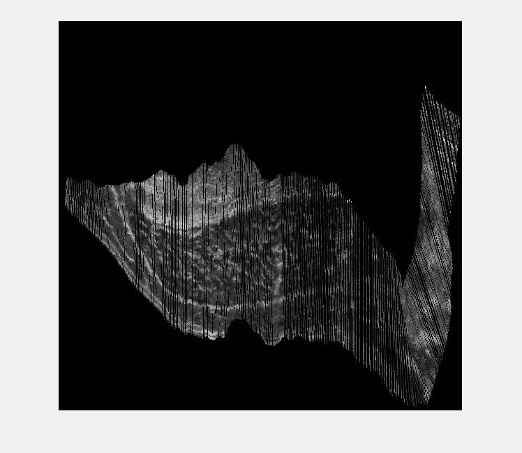
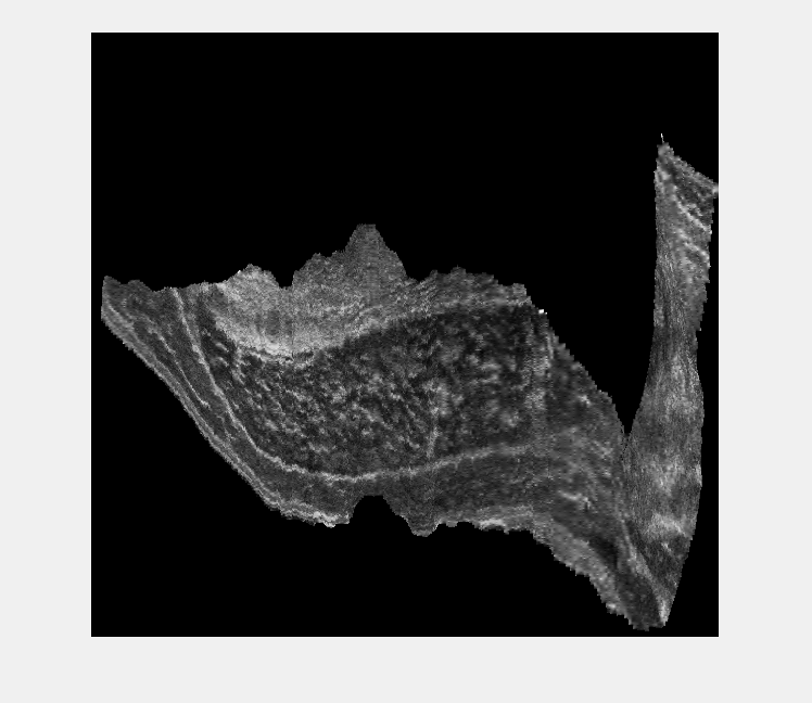
vii. Imaging and anatomical knowledge: Another important consideration in using any imaging modality is that the knowledge of both the anatomy and the imaging modality is essential to obtain meaningful interpretation. Anatomical variation between subjects and image artifacts needs to be recognized and taken into account in the identification process of anatomical structures. Even with healthy and/or well developed muscles, clear identification can be difficult because it requires anatomical knowledge to differentiate between different components of one muscle or between muscle groups51. However, in atrophied muscle (i.e. elderly, in the case of pathology, or a cadaver), the clear identification is even more complicated because of a smaller size and decreased image contrast, and therefore less distinct tissue interfaces (Figure 4). We believe that without prior anatomical knowledge, we would have been limited in making correct judgements in designing this 3DUS approach and in performing the 3DUS measurements. For example, for GM experiments, different footplate angles do not necessarily cause expected changes in muscle tendon complex lengths, due to deformation within the foot7. Also detailed anatomical information on curvature of the distal aponeurosis was essential for an adequate selection of the mid-longitudinal plane in all subjects38.

Figure 4: Variation and quality of reconstructed anatomical cross-sectional 3DUS images of the quadriceps muscle halfway along the thigh. (A) Example of a male human cadaver shows an image of an atrophied state at death (death age: 81 years). Identification of the boundaries of individual heads of the quadriceps muscle is difficult. (B) Example of a sedentary male (aged 30 years). (C) Example of a male athlete rower (aged 30 years). The white squares for scale represent 1 cm x 1 cm. Please click here to view a larger version of this figure.
Future Applications:
The 3DUS approach provides an imaging tool that can be used for various purposes and settings in sports and clinics. In clinical interventions effectiveness is related to the physical fitness level52. Using 3DUS for monitoring patients who are at risk of losing muscle mass is important (e.g., references53,54,55) and potentially allows for adjustment of the treatment. Another potential application of 3DUS lies in monitoring the morphological adaptation of muscle in response to intervention (training) and/or injury.
This protocol described a cost- and time-effective method of measuring soft tissue structure of the human body based on freehand 3DUS sweeps. Moreover, assessment of the meaningful morphological parameters of m. vastus lateralis and m. gastrocnemius medialis proved to be valid and reliable.
Disclosures
The authors have nothing to disclose.
Acknowledgments
The authors are very grateful to Adam Shortland and Nicola Fry who shared their algorithms for the 3-dimensional ultrasound in 2004, which were the inspiration for the development of the software used in this study.
Materials
| Name | Company | Catalog Number | Comments |
| Ultrasound device (Technos MPX) | Esaote, Italy | NA | |
| Linear array probe (12.5 Mhz, 5 cm) | Esaote, Italy | NA | |
| Workstation (HP Z440) | HP, USA | http://www8.hp.com/us/en/workstations/z440.html | |
| Framegrabber (Canopus, ADVC 300) | Canopus, Japan | ADVC 300 | |
| Motion Capture System (Certus) | NDI, Canada | http://www.ndigital.com/msci/products/optotrak-certus/ | |
| Synchronisation device | VU, NL | Contact corresponding author | |
| Calibration frame | VU, NL | Contact corresponding author | |
| Thermometer | Greisinger, Germarny | GTH 175/PT | |
| Examination table | NA | NA | Any examination table |
| Inclinometer | Lafayette instrument, USA | ACU001 | |
| Adjustable Footplate | VU, NL | Contact corresponding author | |
| Torque wrench | VU, NL | Contact corresponding author | |
| Extendable rod | VU, NL | Contact corresponding author | |
| Goniometer (Gollehon) | Lafayette instrument, USA | 1135 | |
| Triangular shaped beam | NA | NA | Made out a piece of stiff foam |
| Lashing straps | NA | NA | Any lashing strap |
| Surgical skin marker | NA | NA | Any surgical skin marker |
| Ultrasound transmission gel | Servoson | NA | A sticky gel type is recommended |
References
- Reeves, N. D., Maganaris, C. N., Narici, M. V. Ultrasonographic assessment of human skeletal muscle size. Eur. J. Appl. Physiol. 91, 116-118 (2004).
- Van Den Engel-Hoek, L., Van Alfen, N., De Swart, B. J. M., De Groot, I. J. M., Pillen, S. Quantitative ultrasound of the tongue and submental muscles in children and young adults. Muscle Nerve. 46, 31-37 (2012).
- Seymour, J. M., et al. Ultrasound measurement of rectus femoris cross-sectional area and the relationship with quadriceps strength in COPD. Thorax. 64, 418-423 (2009).
- Seymour, J. M., et al. The prevalence of quadriceps weakness in COPD and the relationship with disease severity. Eur. Respir. J. 36, 81-88 (2010).
- Ho, S. S. Y. Current status of carotid ultrasound in atherosclerosis. Quant. Imaging Med. Surg. 6, 285-296 (2016).
- Barber, L., Barrett, R., Lichtwark, G. Passive muscle mechanical properties of the medial gastrocnemius in young adults with spastic cerebral palsy. J. Biomech. 44, 2496-2500 (2011).
- Huijing, P. A., Bénard, M. R., Harlaar, J., Jaspers, R. T., Becher, J. G. Movement within foot and ankle joint in children with spastic cerebral palsy: a 3-dimensional ultrasound analysis of medial gastrocnemius length with correction for effects of foot deformation. BMC Musculoskelet. Disord. 14, 365 (2013).
- Shortland, A. P., Harris, C. A., Gough, M., Robinson, R. O. Architecture of the medial gastrocnemius in children with spastic diplegia. Dev. Med. Child Neurol. 44, 158-163 (2002).
- Farup, J., et al. Muscle Morphological and Strength Adaptations to Endurance Vs. Resistance Training. J. Strength Cond. Res. 26, 398-407 (2012).
- Timmins, R. G., Shield, A. J., Williams, M. D., Lorenzen, C., Opar, D. A. Architectural adaptations of muscle to training and injury: a narrative review outlinig the contributions by fascicle lenght, pennation angle and muscle thickness. Br. J. Sports Med. 0, 1-7 (2016).
- Huijing, P. Important experimental factors for skeletal muscle modelling: non-linear changes of muscle length force characteristics as a function of degree of activity. Eur. J. Morphol. 34, 47-54 (1996).
- Van der Linden, B., Koopman, H., Grootenboer, H. J., Huijing, P. A. Modelling functional effects of muscle geometry. J. Electromyogr. Kinesiol. 8, 101-109 (1998).
- Woittiez, R. D., Huijing, P. A., Boom, H. B., Rozendal, R. H. A three-dimensional muscle model: a quantified relation between form and function of skeletal muscles. J. Morphol. 182, 95-113 (1984).
- Lieber, R. L., Blevins, F. T. Skeletal muscle architecture of the rabbit hindlimb: functional implications of muscle design. J. Morphol. 199, 93-101 (1989).
- Weide, G., et al. Medial gastrocnemius muscle growth during adolescence is mediated by increased fascicle diameter rather than by longitudinal fascicle growth. J. Anat. 226, 530-541 (2015).
- Fukunaga, T., et al. Physiological cross-sectional area of human leg muscles based on magnetic resonance imaging. J. Orthop. Res. 10, 926-934 (1992).
- LeBlanc, A., et al. Muscle volume, MRI relaxation times (T2), and body composition after spaceflight. J. Appl. Physiol. 89, (2000).
- Lindemann, U., et al. Association between Thigh Muscle Volume and Leg Muscle Power in Older Women. PLoS One. 11, 0157885 (2016).
- Gopalakrishnan, R., et al. Muscle Volume, Strength, Endurance, and Exercise Loads During 6-Month Missions in Space. Aviat. Space. Environ. Med. 81, 91-104 (2010).
- Wakahara, T., Ema, R., Miyamoto, N., Kawakami, Y. Inter- and intramuscular differences in training-induced hypertrophy of the quadriceps femoris: association with muscle activation during the first training session. Clin. Physiol. Funct. Imaging. , (2015).
- Pamuk, U., Karakuzu, A., Ozturk, C., Acar, B., Yucesoy, C. A. Combined magnetic resonance and diffusion tensor imaging analyses provide a powerful tool for in vivo assessment of deformation along human muscle fibers. J. Mech. Behav. Biomed. Mater. 63, 207-219 (2016).
- Prager, R. W., Rohling, R. N., Gee, A. H., Berman, L. Rapid calibration for 3-D freehand ultrasound. Ultrasound Med. Biol. 24, 855-869 (1998).
- Solberg, O. V., Lindseth, F., Torp, H., Blake, R. E., Nagelhus Hernes, T. A. Freehand 3D Ultrasound Reconstruction Algorithms-A Review. Ultrasound Med. Biol. 33, 991-1009 (2007).
- Gee, A., Prager, R., Treece, G., Berman, L. Engineering a freehand 3D ultrasound system. Pattern Recognition Letters. 24, (2003).
- Bénard, M. R., Harlaar, J., Becher, J. G., Huijing, P. A., Jaspers, R. T. Effects of growth on geometry of gastrocnemius muscle in children: a three-dimensional ultrasound analysis. J. Anat. 219, 388-402 (2011).
- Fry, N. R., Gough, M., Shortland, A. P. Three-dimensional realisation of muscle morphology and architecture using ultrasound. Gait Posture. 20, 177-182 (2004).
- Barber, L., Barrett, R., Lichtwark, G. Passive muscle mechanical properties of the medial gastrocnemius in young adults with spastic cerebral palsy. J. Biomech. 44, 2496-2500 (2011).
- MacGillivray, T. J., Ross, E., Simpson, H. A. H. R. W., Greig, C. A. 3D Freehand Ultrasound for in vivo Determination of Human Skeletal Muscle Volume. Ultrasound Med. Biol. 35, 928-935 (2009).
- Rana, M., Wakeling, J. M. In-vivo determination of 3D muscle architecture of human muscle using free hand ultrasound. J. Biomech. 44, 2129-2135 (2011).
- Haberfehlner, H., et al. Freehand three-dimensional ultrasound to assess semitendinosus muscle morphology. J. Anat. 229, 591-599 (2016).
- Bénard, M. R., Jaspers, R. T., Huijing, P. A., Becher, J. G., Harlaar, J. Reproducibility of hand-held ankle dynamometry to measure altered ankle moment-angle characteristics in children with spastic cerebral palsy. Clin Biomech. 25, 802-808 (2010).
- de Ruiter, C. J., Kooistra, R. D., Paalman, M. I., de Haan, A. Initial phase of maximal voluntary and electrically stimulated knee extension torque development at different knee angles. J. Appl. Physiol. 97, (2004).
- Kooistra, R. D., de Ruiter, C. J., de Haan, A. Knee angle-dependent oxygen consumption of human quadriceps muscles during maximal voluntary and electrically evoked contractions. Eur. J. Appl. Physiol. 102, 233-242 (2008).
- WinDV. , Available from: http://windv.mourek.cz/le (2017).
- VirtualDub. , Available from: http://virtualdub.org (2017).
- D'Errico, J. inpaint_nans. Matlab Central File Exchange. , Available from: www.mathworks.com/matlabcentral/fileexchange/4551 (2004).
- MITK. , Available from: http://mitk.org/wiki/MITK (2004).
- Bénard, M. R., Becher, J. G., Harlaar, J., Huijing, P. A., Jaspers, R. T. Anatomical information is needed in ultrasound imaging of muscle to avoid potentially substantial errors in measurement of muscle geometry. Muscle Nerve. 39, 652-665 (2009).
- Fix for Life Embalming. , Available from: www.fixforlifeembalming.com (2017).
- ImageJ. , Available from: https://fiji.sc (2017).
- Weir, J. P. Quantifying test-retest reliability using the intraclass correlation coefficient and the SEM. J. Strength Cond. Res. 19, 231-240 (2005).
- Prager, R. W., Gee, A., Berman, L. Stradx: real-time acquisition and visualization of freehand three-dimensional ultrasound. Med. Image Anal. 3, 129-140 (1999).
- Solberg, O. V., Lindseth, F., Torp, H., Blake, R. E., Nagelhus Hernes, T. A. Freehand 3D Ultrasound Reconstruction Algorithms-A Review. Ultrasound in Medicine and Biology. 33, 991-1009 (2007).
- Mitsiopoulos, N., et al. Cadaver validation of skeletal muscle measurement by magnetic resonance imaging and computerized tomography. J. Appl. Physiol. 85, (1998).
- Jackowski, C., et al. Noninvasive Estimation of Organ Weights by Postmortem Magnetic Resonance Imaging and Multislice Computed Tomography. Invest. Radiol. 41, 572-578 (2006).
- Weller, R., et al. The Determination of Muscle Volume with A Freehand 3D Ultrasonography System. Ultrasound Med. Biol. 33, 402-407 (2007).
- Barber, L., Barrett, R., Lichtwark, G. Validation of a freehand 3D ultrasound system for morphological measures of the medial gastrocnemius muscle. J. Biomech. 42, 1313-1319 (2009).
- Delcker, A., Walker, F., Caress, J., Hunt, C., Tegeler, C. In vitro measurement of muscle volume with 3-dimensional ultrasound. Eur J. Ultrasound. 9, (1999).
- Cenni, F., et al. The reliability and validity of a clinical 3D freehand ultrasound system. Comput. Methods Programs Biomed. 136, 179-187 (2016).
- de Brito Fontana, H., Herzog, W. Vastus lateralis maximum force-generating potential occurs at optimal fascicle length regardless of activation level. Eur. J. Appl. Physiol. 116, 1267-1277 (2016).
- Engstrom, C. M., Loeb, G. E., Reid, J. G., Forrest, W. J., Avruch, L. Morphometry of the human thigh muscles. A comparison between anatomical sections and computer tomographic and magnetic resonance images. J. Anat. 176, 139-156 (1991).
- Warburton, D. E. R., Nicol, C. W., Bredin, S. S. D. Health benefits of physical activity: the evidence. CMAJ. 174, 801-809 (2006).
- Moisey, L. L., et al. Skeletal muscle predicts ventilator-free days, ICU-free days, and mortality in elderly ICU patients. Crit. Care. 17, 206 (2013).
- Weijs, P. J., et al. Low skeletal muscle area is a risk factor for mortality in mechanically ventilated critically ill patients. Crit. Care. 18, 12 (2014).
- English, K. L., Paddon-Jones, D. Protecting muscle mass and function in older adults during bed rest. Curr. Opin. Clin. Nutr. Metab. Care. 13, 34-39 (2010).
