

Summary
Electrochemical impedance spectroscopy (EIS) of species that undergo reversible oxidation or reduction in solution was used for determination of rate constants of oxidation or reduction.
Abstract
Electrochemical impedance spectroscopy (EIS) was used for advanced characterization of organic electroactive compounds along with cyclic voltammetry (CV). In the case of fast reversible electrochemical processes, current is predominantly affected by the rate of diffusion, which is the slowest and limiting stage. EIS is a powerful technique that allows separate analysis of stages of charge transfer that have different AC frequency response. The capability of the method was used to extract the value of charge transfer resistance, which characterizes the rate of charge exchange on the electrode-solution interface. The application of this technique is broad, from biochemistry up to organic electronics. In this work, we are presenting the method of analysis of organic compounds for optoelectronic applications.
Introduction
Redox rate of the electroactive compound is an important parameter characterizing its ability to undergo oxidation or reduction processes and predict its behavior in the presence of strong oxidizing or reducing agents or under applied potential. However, most of the electrochemical techniques are only able to qualitatively describe the kinetics of the redox process. Among various electrochemical techniques employed for redox active compounds, characterization cyclic voltammetry (CV) is the most prevailing method for quick and sufficient electrochemical characterization of various soluble species1,2,3. The CV technique has broad applications, e.g., energy levels estimations4,5,6, the charge carriers analysis supported by spectroscopies7,8,9,10, up to surface modifications11,12,13. Like every method, CV is not perfect and to increase the applicability and quality of results, the connection with another spectroscopic technique is important. We already present several investigations where the electrochemical impedance spectroscopy (EIS) technique was employed14,15,16 but in this work, we intended to show step-by-step how to reinforce the CV technique by EIS.
The EIS output signal consists of two parameters: real and imaginary parts of impedance as functions of frequency17,18,19,20. It allows estimation of several parameters responsible for charge transfer through the electrode-solution interface: double layer capacitance, solution resistance, charge transfer resistance, diffusion impedance and other parameters depending on system investigated. Charge transfer resistance was an object of high attention since this parameter is directly related to the redox rate constant. Even though oxidation and reduction rate constants are estimated in solution, they may generally characterize the ability of a compound for charge exchange. EIS is considered to be an advanced electrochemical technique requiring profound mathematical understanding. Its main principles are described in modern electrochemistry literature17,18,19,20,21,22,23.
Protocol
1. Basic Preparation of an Electrochemical Experiment
- Prepare 4 mL of a working solution containing 0.1 mol∙L−1 Bu4NBF4 and 0.001 mol∙L−1 investigated organic compound by adding calculated amounts of solid powders into 4 mL of dichloromethane in a small vessel or a test tube. With 2,8-bis(3,7-dibutyl-10H-phenoxazin-10- yl)dibenzo[b,d]thiophene-S,S-dioxide (molar mass 802 g∙mol−1), weigh 3.208 mg of this compound and 0.1645 g of Bu4NBF4.
- Fill a 3 mL electrochemical cell with 2 mL of solution using a pipette. The remaining portion of the solution will be needed later for impedance measurement and reproducing the results.
- Polish a 1 mm diameter platinum working disc electrode (WE) for 30 s using a polishing cloth moistened by several drops of alumina slurry. Rub the flat surface of the disc electrode with a piece of cloth mounted on an immobile support (e.g. Petri dish) by applying moderate pressure.
- Rinse the electrode with distilled water three times to remove alumina particles.
- Anneal a counter electrode (CE, platinum wire) in a butane burner flame. Carefully put the platinum wire in a flame for less than 1 s and quickly remove when it starts reddening to avoid melting.
NOTE: The CE surface area is not stipulated but must be much higher than the surface area of the working electrode. In this case, impedance of working electrode interface would have the major impact on the total system impedance and would permit excluding counter electrode impedance from consideration.- Anneal a reference electrode (RE, silver wire) in butane burner flame in the same manner.
- Put all three electrodes (working, counter and reference) into a cell avoiding mutual contact and connect to the corresponding potentiostat cables marked as WE, CE and RE. Insert a gas delivering tube connected with argon gas bottle for further deaeration.
- Open the gas valve and deaerate solution by bubbling argon through the solution for 20 min. Close the gas valve before measurement.
2. Tentative Characterization by Cyclic Voltammetry (CVA)
- Register the CVA of the working solution within a potential range from −2.0 V to +2.0 V and scan rate 100 mV∙s−1.
- Launch the program Cyclic voltammetry in the potentiostat software.
- Choose 0.0 V as initial potential value, −2.0 V as minimal potential, +2.0 V as maximal scanning potential, 100 mV∙s−1 as scanning rate. Other parameters are optional.
- Click the button Start.
NOTE: A typical voltammogram is presented in Figure 1.
- Determine the potential value from the CVA obtained. Note the potential values when maxima of positive (anodic peak) and negative (cathodic peak) current appear and calculate the average value.
- Add 10 mg of ferrocene by spatula into the working solution and deaerate it by argon bubbling for 5 min. This is necessary for mixing and complete dissolution of the ferrocene added.
NOTE: The ferrocene amount is not precise. However, adding less than 1 mg or more than 20 mg would complicate estimation of equilibrium potential. - Register the CVA of the working solution within the potential range from −1.0 V to +1.0 V and scan rate 100 mV∙s−1. A small reversible peak of ferrocene will appear as shown in Figure 1.
- Determine the potential value of ferrocene reversible oxidation from the CVA obtained. Note the potential values when maxima of positive (anodic peak) and negative (cathodic peak) current appear and calculate the average value.
- Put another portion of the solution prepared at step 1.1 into the cell and clean the electrodes by repeating the procedure described in 1.2-1.7.
3. Registration of Impedance Spectrum
NOTE: An example of the setup in software is shown in Figure 2; any other software or device also can be used. However, the setup arrangement may differ in different software, although the main principles remain the same. Use the EIS in a staircase mode, i.e. potentiostatic spectra are registered automatically one after another.
- In the software, choose a potential range of 0.2 V covering the reversible peak in CVA. Example: A reversible oxidation peak was detected on CV at 0.7 V. The potential range for CV should be then from 0.6 V to 0.8 V. The spectra will be registered with the increment of 0.01 V, i.e. at 0.61 V, 0.62 V, etc.
- Register the EIS automatic measurement procedure under following conditions advised.
- Enter the following input values: initial potential 0.6 V; finish potential 0.8 V; potential increment: 0.01 V; frequency range: from 10 kHz through 100 Hz; the number of frequencies in logarithmic scale: 20; wait for a time between the spectra: 5 s, ac voltage amplitude 10 mV, minimal 2 measures per frequency.
- Click the button Start.
NOTE: In that case, 21 spectra, each containing 41 frequency points will be obtained. The typical set of automatically registered spectra is presented in Figure 3.
4. Analysis of Impedance Spectrum
- Launch the program EIS spectrum analyser.
- Download the spectrum by choosing File | Open.
- In the right upper sub-window construct an EEC by using left/right mouse click choosing series or parallel connection and necessary element from the context menu: C - capacitor, R - resistor, W - Warburg element. Start from the simplest circuit (Figure 5c).
- Choose initial minimal and maximal values for parameters by left-mouse-clicking table cells and entering values: C1 - from 1∙10-7 to 1∙10-8, R1 - from 2000 to 100, R2 - from 1000 to 100, Aw - from 50000 to 10000.
- Fit the model by choosing Model | Fit. Repeat the procedure several times (usually about 5 times) until the calculated values no longer change. Parameter values are shown in a table in the upper left sub-window.
- Check parameter errors shown in the last column of the table. If an error of a parameter exceeds 100%, that means that the parameter is not necessary for a circuit. In that case try another equivalent circuit.
NOTE: If one tries to fit an experimental spectrum corresponding to the simple circuit (Figure 5c) by a more complicated circuit (Figure 5a), then errors of unnecessary additional parameters W and R3 would be considerably high. - Check the values of r2(parametric) and r2(amplitude) presented in the lower right sub-window. If they exceed limit 1∙10−2, repeat the procedures 4.2−4.5 using another equivalent electrical circuit (EEC) (Figure 5).
- Repeat the procedure 4.1-4.7 for all the spectra registered
- For each spectrum analyzed, write down the calculated value of charge transfer resistance and the corresponding potential that the spectrum was registered at.
5. Calculation of Redox Rate Constants
- Put the values of the estimated inverse charge transfer resistance versus potential. A typical potential plot of inverse charge transfer resistance for the reversible process is presented in Figure 6.
- Open an empty sheet of spreadsheet software.
- Manually enter the values of potentials and corresponding values of reverse charge transfer resistance in columns A and B.
- Select the range A1:B21 and choose Insert | Graph | Pointed by mouse clicking in the task menu.
- Plot the values of a theoretical function calculated by the formula (1) on the same plot. Use constant values: F = 96485 C∙mol−1, c0 = 0.01 mol∙−1, z = 1, R = 8.314 J∙mol−1∙K−1, α = 0.5, T - ambient temperature. Use the previously estimated value (3.1) of E0.
 (1)
(1)
 (2)
(2)
where Rct−1 is inverse value of charge transfer resistance normalized by surface area; z- number of electrons transferred in one step (accepted being equal 1); F- Faraday constant; c0- concentration of investigated compound; α - charge transfer coefficient (accepted being equal 0.5); E- electrode potential; parameter θ was introduced to simplify the final formula relating E and Rct.- Copy the first column of values (potential values) in the same sheet in column D.
- Enter the constant values of F, c0, z, R, α, T, E0, k0 enlisted above into cells C1:C8. Use values E0 = 0, k0 = 1∙10−5.
- Enter formula (2) to calculate θ into cell E1: =EXP($C$1*$C$3/($C$4*$C$6)*(D1-$C$7)).
- Copy the formula into cells E2:E21 by selecting E1, clicking Copy, selecting range E2:E21 and clicking Paste.
- Enter formula (1) into cell F1: = $C$8*$C$1^2*$C$3^2/($C$4*$C$6)*$C$2*E1^(1-$C$5)/(1+E1).
- Copy the formula into cells F2:F21 by selecting F1, clicking Copy, selecting range F2:F21 and clicking Paste.
- Left click on the graph built at step 5.1, choose Choose data, then Add and add new data set by specifying entering D1:D21 as x range and F1:F21 as y range.
NOTE: Two graphs: experimental and simulated automatically marked by different colors will appear on one coordinate plot.
- Optimize the theoretical function (1) in order to fir experimental data by varying values of equilibrium potential (E0) and standard rate constant (k0), being the target parameter.
NOTE: Change of the values in cells C7 (E0) and C8 (k0) would immediately cause change of the simulated graph.- Change values in cells C7 and C8 manually in order to achieve equality between experimental and simulated graph.
NOTE: Change of E0 moves the bell-like curve along the x axis. Change of k0 controls the height of the bell-like curve. Thus, varying those two only parameters can be used to find a theoretical model corresponding to experimental results (Figure 6). Parameter α (1) controls symmetry of theoretical peak. However, in real systems asymmetry may be caused by the occurrence of side-process rather than by α. Since it influences resulting k0 value we recommend not to manipulate α value and leave it to equal 0.5.
- Change values in cells C7 and C8 manually in order to achieve equality between experimental and simulated graph.
 (1)
(1) (2)
(2)Representative Results
The first step is cyclic voltammetry characterization presented in Figure 1. Application of EIS was successful when compounds underwent the fast reversible electrochemical process. Such behavior was often not observed for organic compounds but organic compounds that possess electroconductivity in a solid state was found to be a good specimen for electrochemical kinetic investigation. One such organic compound is shown in the inset of Figure 1.
Registration of impedance spectra was carried out according to the experimental setup (Figure 2), and typical raw resulting data are shown in Figure 3. Analysis of impedance spectra was carried out using special software24. The window of the open access program EIS Spectrum analyser24 during results processing is shown in Figure 4. An EEC used to fit the spectrum is built manually in the right upper sub-window. The calculated EEC parameters (resistances R1 and R2, capacitance C1 and diffusion impedance parameter W1) are shown in a table in the left upper sub-window. The graph in lower left sub-window illustrates fitting of experimental results (red points) with the theoretically calculated data plot (green line).
Several different EEC may fit experimental spectrum depending on the processes that take place on the electrode surface and their rates (Figure 5). The simplest semi-infinite Warburg element can be used as there is no distortion of solution (e.g. rotating of the electrode mixing) and no electrode coating limiting the diffusion. In case of considerably fast electrochemical reactions, resistance R3 (Figure 5A) was high enough to be neglected in comparison with other parallel branches of EEC (Figure 5B). Moreover, when rate of charge transfer (R2) is significantly higher than diffusion, the charge transfer step becomes limiting and an even simpler EEC (Figure 5C) describes the system.
The series resistor R1 is always present in EEC. It corresponds to the external resistance including connectors and solution, except electrode-surface interface. Capacitor C1 characterizes a double layer formed at the electrode interface. The branch including resistor and Warburg element diffusion impedance (Figure 5A) corresponds to a fast electrochemical process including two stages: kinetic and diffusion, respectively. The third resistor corresponds to a slower electrochemical process that takes place on the electrode surface and involves solvent or molecules that have undergone fast oxidation or reduction. In some cases, parameters, R3 and W1 were impossible to estimate. Then they might be considered as absent and not taken into account as Figure 5B and 5C show.
Although EIS provides an estimation of several parameters, the target element which is considered in this work is charge transfer resistor R2 usually assigned as Rct in literature17,18,19, which stands in parallel to the capacitor and in series to Warburg element. Its dependence on voltage is shown in Figure 6.
According to the theory of electrochemical kinetics (Protocol, step 5.2), charge transfer resistance is directly related to the standard electrochemical rate constant. Even though matching between experimental and theoretical results was not ideal, it allowed estimation of the value of the standard electrochemical rate constant and defined the value of equilibrium potential by maximum position.
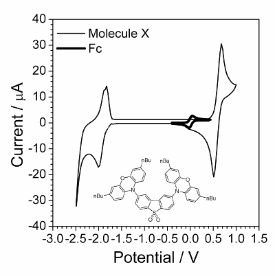
Figure 1: Cyclic voltammogram of investigated compound overlapped by cyclic voltammogram in presence of small amount of ferrocene. Solution: 1.0 mol∙L−1 Bu4NBF4 and 0.01 mol∙L−1 X in dichloromethane. Structure of compound X (2,8-bis(3,7-dibutyl-10H-phenoxazin-10-yl)dibenzo[b,d]thiophene-S,S-dioxide) is shown in the inset. Please click here to view a larger version of this figure.

Figure 2: Experimental setup controlling registration of 20 spectra within the voltage range from 0.6 to 0.8 V in the frequency range from 10 kHz to 100 Hz with 20 points for each decade. Ei, Ef- initial and final potentials respectively, N - number of steps, ts- waiting time before each measurement, dt - record time interval, fi, ff- initial and final frequency, ND- number of frequency points in one spectrum, Va- ac amplitude, pw - part of time in respect to one point registration used to switch to another frequency, Na- number of measurements at one frequency, E range, I range, Bandwidth - technical parameters. Please click here to view a larger version of this figure.

Figure 3: Scan of screen during impedance spectra registration. Upper right sub-window: staircase dependence of electrode potential on time. Upper left sub-window: Nyquist plot, imaginary impedance (ordinate), real impedance (abciss). Lower left sub-window: Bode plot, impedance module (left scale), phase shift (right scale), frequency (horizontal scale). Please click here to view a larger version of this figure.

Figure 4: «EIS Spectrum analyzer» program window during results processing. Upper left sub-window: parameter values table: C1 - capacitance, R1, R2 - resistances, W1 - Warburg element; lower left sub-window: experimental (green points) and theoretical model (red line) spectra; upper right sub-window: equivalent electrical circuit; lower right sub-window: calculated statistics of fitting. Please click here to view a larger version of this figure.

Figure 5: Equivalent electrical circuits found to fit the impedance spectra of redox processes on the electrode surface. (A) - reversible electrochemical process accompanied by parallel irreversible process, (B) - reversible electrochemical process, (C) - electrochemical process with kinetic limitation stage. Please click here to view a larger version of this figure.

Figure 6: Inverse values of charge transfer resistance estimated from EIS versus electrode potential. The line depicts theoretically predicted dependence according to formula (2).
Discussion
This part of the work will be devoted to an explanation of chosen experimental conditions and discussion of possible applications of the method presented.
Analysis of impedance spectrum may be performed by various software. Here the basic recommendations for EEC analysis method are discussed. One needs to know that there are numerous fitting algorithms and various ways of error estimation. We present an example of using open access software developed by A. Bondarenko and G. Ragoisha24 (Figure 4).
Exact estimation of Rct value was the main objective of the work. One of the reasons for the choice of the experimental conditions was an intention to conceal the impact of diffusion. Thus, the solution concentration had to be as high as possible. While acquiring the experimental results shown here, the concentration was limited due to economic reasons. The range of frequencies from 10 kHz to 100 Hz was chosen to eliminate the effect of diffusion as well. Diffusion impedance is inversely proportional to the frequency while resistance is not dependent on the frequency. The effect of resistance in the high-frequency part of the spectrum was higher than in the low-frequency part. Spectra were not registered at the frequencies lower than 100 Hz because these data would be useless for resistance calculation. All the electrochemical results obtained in non-aqueous solvent are presented versus ferrocene-oxidized / ferrocene coupled equilibrium potential. For this reason, steps 2.3 - 2.5 are performed.
We considered EIS application to organic molecules characterization. Analysis of other EEC parameters and their potential dependencies in perspective may lead to the revelation of other effects and electrochemical characterization of compounds in solution. Estimation of redox rate constants is useful for describing the kinetics of electroactive compound reduction or oxidation and predicting material behavior in oxidizing or reducing medium.
Disclosures
The authors have nothing to disclose.
Acknowledgments
The authors gratefully acknowledge the financial support of "Excilight" project "Donor-Acceptor Light Emitting Exciplexes as Materials for Easy-to-tailor Ultra-efficient OLED Lightning" (H2020-MSCA-ITN-2015/674990) financed by Marie Skłodowska-Curie Actions within the framework programme for research and innovations "Horizon-2020".
Materials
| Name | Company | Catalog Number | Comments |
| Potentiostat | BioLogic | SP-150 | |
| Platinum disc electrode | eDAQ | ET075 | 1 mm diameter |
| Platinum wire | − | − | counter electrode |
| Silver wire | − | − | silver electrode |
| Electrochemical cell | eDAQ | ET080 | 3 mL volume |
| Polishing cloth | eDAQ | ET030 | |
| Alumina slurry | eDAQ | ET033 | 0.05 µm |
| Butane torch | Portasol | Mini-Torch/Heat Gun | |
| Dichloromethane (DCM) | Sigma-Aldrich | 106048 | |
| Tetrabutylammonium tetrafluoroborate (Bu4NBF4) | Sigma-Aldrich | 86896 |
References
- Cunningham, A. J., Underwood, A. L. Cyclic Voltammetry of the Pyridine Nucleotides and a Series of Nicotinamide Model Compounds. Biochemistry. 6, 266-271 (1967).
- Laba, K., et al. Diquinoline derivatives as materials for potential optoelectronic applications. J Phys Chem C. 119, 13129-13137 (2015).
- Data, P., Lapkowski, M., Motyka, M., Suwinski, J. Electrochemistry and spectroelectrochemistry of a novel selenophene-based monomer. Electrochim Acta. 59, 567-572 (2012).
- Laba, K., et al. Electrochemically induced synthesis of poly(2,6-carbazole). Macromol Rapid Commun. 36, 1749-1755 (2015).
- Data, P., Lapkowski, M., Motyka, M., Suwinski, J. Influence of alkyl chain on electrochemical and spectroscopic properties of polyselenophenes. Electrochim Acta. 87, 438-449 (2013).
- Data, P., Lapkowski, M., Motyka, M., Suwinski, J. Influence of heteroaryl group on electrochemical and spectroscopic properties of conjugated polymers. Electrochim Acta. 83, 271-282 (2012).
- Gora, M., et al. EPR and UV-vis spectroelectrochemical studies of diketopyrrolopyrroles disubstituted with alkylated thiophenes. Synth Met. 216, 75-82 (2016).
- Pluczyk, S., Zassowski, P., Quinton, C., Audebert, P., Alain-Rizzo, V., Lapkowski, M. Unusual Electrochemical Properties of the Electropolymerized Thin Layer Based on a s-Tetrazine-Triphenylamine Monomer. J Phys Chem C. 120, 4382-4391 (2016).
- Data, P., Motyka, M., Lapkowski, M., Suwinski, J., Monkman, A. Spectroelectrochemical Analysis of Charge Carries as a Way of Improving Poly(p-phenylene) Based Electrochromic Windows. J Phys Chem C. 119, 20188-20200 (2015).
- Enengl, S., et al. Spectroscopic characterization of charge carriers of the organic semiconductor quinacridone compared with pentacene during redox reactions. J Mater Chem C. 4, 10265-10278 (2016).
- Piwowar, K., Blacha-Grzechnik, A., Turczyn, R., Zak, J. Electropolymerized phenothiazines for the photochemical generation of singlet oxygen. Electrochim Acta. 141, 182-188 (2014).
- Blacha-Grzechnik, A., Turczyn, R., Burek, M., Zak, J. In situ Raman spectroscopic studies on potential-induced structural changes in polyaniline thin films synthesized via surface-initiated electropolymerization on covalently modified gold surface. Vib Spectrosc. 71, 30-36 (2014).
- Blacha-Grzechnik, A., et al. Phenothiazines grafted on the electrode surface from diazonium salts as molecular layers for photochemical generation of singlet oxygen. Electrochim Acta. 182, 1085-1092 (2015).
- Data, P., et al. Evidence for Solid State Electrochemical Degradation Within a Small Molecule OLED. Electrochim Acta. 184, 86-93 (2015).
- Data, P., et al. Electrochemically Induced Synthesis of Triphenylamine-based Polyhydrazones. Electrochim Acta. 230, 10-21 (2017).
- Data, P., et al. Kesterite Inorganic-Organic Heterojunction for Solution Processable Solar Cells. Electrochim Acta. 201, 78-85 (2016).
- Barsoukov, E., Macdonald, J. R. Impedance Spectroscopy: Theory, Experiment, and Applications. , Wiley. (2005).
- Orazem, M. E., Tribollet, B. Electrochemical Impedance Spectroscopy. , Wiley. (2008).
- Lasia, A. Electrochemical Impedance Spectroscopy and its Applications. , Springer. (2014).
- Bard, A. J., Faulkner, L. R. Electrochemical Methods: Fundamentals and Applications. , Wiley. (2013).
- Scholz, F. Electroanalytical methods: Guide to Experiment and Application. , Springer. (2010).
- Conway, B. E., Bockris, J. O. 'M., White, R. E. Modern Aspects of Electrochemistry. 32, Kluwer Academic Publishers. (2002).
- Encyclopedia of Electrochemistry: V. 3. Instrumentation and Electroanalytical Chemistry. Bard, A. J., Starttman, M., Unwin, P. R. , Wiley. (2003).
- EIS spectrum analyser software. , Available from: http://www.abc.chemistry.bsu.by/vi/analyser (2017).
