An Analog Macroscopic Technique for Studying Molecular Hydrodynamic Processes in Dense Gases and Liquids

Summary

An experimentally accessible analog method for studying molecular hydrodynamic processes in dense fluids is presented. The technique uses particle image velocimetry of vibrated, high-restitution grain piles and allows direct, macroscopic observation of dynamical processes known and predicted to exist in strongly interacting, high density gases and liquids.

Abstract

An analog, macroscopic method for studying molecular-scale hydrodynamic processes in dense gases and liquids is described. The technique applies a standard fluid dynamic diagnostic, particle image velocimetry (PIV), to measure: i) velocities of individual particles (grains), extant on short, grain-collision time-scales, ii) velocities of systems of particles, on both short collision-time- and long, continuum-flow-time-scales, iii) collective hydrodynamic modes known to exist in dense molecular fluids, and iv) short- and long-time-scale velocity autocorrelation functions, central to understanding particle-scale dynamics in strongly interacting, dense fluid systems. The basic system is composed of an imaging system, light source, vibrational sensors, vibrational system with a known media, and PIV and analysis software. Required experimental measurements and an outline of the theoretical tools needed when using the analog technique to study molecular-scale hydrodynamic processes are highlighted. The proposed technique provides a relatively straightforward alternative to photonic and neutron beam scattering methods traditionally used in molecular hydrodynamic studies.

Introduction

Molecular hydrodynamics studies the dynamics and statistical mechanics of individual molecules and collections of molecules within fluids. Among the many experimental techniques developed for studying molecular hydrodynamic systems^1,2, light scattering^1,2,3, molecular dynamic simulations^4,5,6,7 and, to a lesser extent, inelastic neutron scattering⁸ have been most commonly used. Unfortunately, significant limitations attach to the latter two techniques. Molecular dynamics (MD) simulations, for example: i) are limited to small spatial and temporal domains containing relatively few molecules , ii) require use of approximate inter-particle potentials, iii) typically introduce periodic boundary conditions, invalid under non-equilibrium bulk flow conditions, and iv) cannot, at present, answer the fundamental question of how molecular-scale dynamics, involving either single molecules or collections of molecules, are affected by, and couple back to, bulk, non-equilibrium fluid flow. The main limitation associated with neutron scattering is tied to the difficulty of accessing the limited number of neutron beam sources available.

In order to provide context for the analog experimental technique presented in this article, we highlight light scattering techniques applied to simple dense-gas and liquid-state fluids. In a typical light scattering experiment, a polarized laser light beam is directed to a small interrogation volume containing a stationary fluid sample. Light scattered from molecules within the sample is then detected at some fixed angle relative to the incident beam. Depending on the molecular dynamic regime of interest, detection and analysis of the scattered light signal incorporates either light filtering or light mixing detection methods. As outlined by Berne and Pecora¹, filtering techniques, which probe fluid state molecular dynamics on time scales shorter than s, introduce a post-scattering interferometer or diffraction grating, and allow scanning of the spectral density of the scattered light. Optical mixing techniques, used for slow-time-scale dynamics, s, by contrast, incorporate a post-scattering autocorrelator or spectrum analyzer, in which the spectral content of the scattered signal is extracted from the measured scattered light intensity.

Generally, laser probes, at least those operating in the visible range of the spectrum, have wavelengths much longer than the characteristic spacing between liquid-state molecules. Under these circumstances, the probe beam excites five collective, slow-time-scale, long-wave-length hydrodynamic modes^2,9,10 (slow relative to the characteristic collision frequency): two viscously damped, counter-propagating sound waves, two uncoupled, purely diffusive vorticity modes, and a single diffusive thermal (entropy) mode. The sound modes are excited in the (longitudinal) direction of the incident beam, while the vortical modes are excited in the transverse direction.

Considering purely experimental scattering techniques, two fundamental questions, lying at the heart of the equilibrium and non-equilibrium statistical mechanics of molecular, liquid-state systems, remain beyond light and neutron scattering measurements:
1) Rigorous arguments^9,11 show that the random, collision- and sub-collision-time-scale dynamics of individual liquid-state molecules, subject to either classical Newtonian dynamics or quantum dynamics, can be recast in the form of generalized Langevin equations (GLE). GLE's, in turn, comprise a central theoretical tool in the study of the non-equilibrium statistical mechanics of molecules in dense gases and liquids. Unfortunately, since the dynamics of individual (non-macromolecular) molecules cannot be resolved by either scattering technique, there is presently no direct way, beyond MD simulations, to test the validity of GLE's.
2) A fundamental hypothesis lying at the heart of macroscopic continuum fluid dynamics, as well microscale molecular hydrodynamics, posits that on length- and time-scales large relative to molecular diameters and collision times, but small relative to continuum length- and time-scales, local thermodynamic equilibrium (LTE) prevails. In continuum flow and heat transfer models, like the Navier-Stokes (NS) equations, the LTE assumption is required⁹ in order to couple intrinsically non-equilibrium, continuum-scale flow and energy transport features — like viscous shear stresses and thermal conduction — to strictly equilibrium thermodynamic properties, like temperature and internal energy. Likewise, while microscale momentum and energy transport are intrinsically non-equilibrium processes, reflecting the appearance of coupled, microscale mass, momentum, and energy currents, models of these microscale processes assume that the currents represent small perturbations from LTE⁹. Again, to the best of our knowledge, there have been no direct experimental tests of the LTE assumption. In particular, it appears that no molecular hydrodynamic scattering experiments have been attempted within dense, moving, non-equilibrium fluid flows.

In this paper, we outline an analog experimental technique in which the macroscopic, single particle and collective particle dynamics of vibrated grain piles, measured using standard Particle Imaging Velocimetry (PIV), can be used to indirectly predict, interpret, and expose single- and multi-molecule hydrodynamics in dense gases and liquids. The physical and theoretical elements that enable the proposed technique are stated in a recent paper published by our group¹². Experimentally, the macroscopic system must exhibit: (i) a sustained tendency toward local, macroscale statistical mechanical equilibrium, and (ii) small, linear departures from equilibrium that mimic (weak) non-equilibrium fluctuations observed in molecular hydrodynamic systems. Theoretically: (i) classical microscale models describing the equilibrium and weakly-non-equilibrium statistical mechanics of dense, interacting N-particle systems must be recast in macroscale form, and (ii) the resulting macroscale models must reliably predict single- and multiple-particle dynamics, from short, particle-collision-time-scales to long, continuum-flow-time-scales.

Here, we present a detailed experimental protocol as well as representative results obtained by the new technique. In contrast to MD simulations and light and neutron scattering methods, the new technique allows, for the first time, detailed study of molecular hydrodynamic processes within flowing, strongly non-equilibrium, dense gases and liquids.

Protocol

1. Preparation of Vibratory System

1. Set up the vibratory system as shown in Figure 1. This system consists of an annular polyurethane bowl (having an outer diameter of 600 mm), attached to a single-speed (1740 rpm), unbalanced motor, where the latter generates process vibrations. This is attached to a weighted base and separated by a group of eight springs (the bowl and weighted base are purchased assembled as one piece). Attach the bowl assembly to its stand and secure with two supplied rubber hooks. Place peristaltic pump on a table near the bowl and attach pump outlet hose to bowl lubrication inlet point.
   1. Attach a triaxial accelerometer to the inner radius of the annular bowl to recorded bowl vibrations under low amplitude conditions and wire the accelerometer to a sensor signal conditioner. Place the signal conditioner on a table away from the vibratory system. The accelerometer/signal conditioner combination is controlled by data acquisition hardware/software installed on a standard computer.
2. Prepare chosen media by washing in water and allowing to dry. Several types of media have been used during various experiments. For this paper, use a ceramic polishing media straight cut triangle (10 mm x 10 mm x 10 mm triangle as viewed from the front and 10 mm thick).
   1. Determine the media packing density by first placing an empty plastic sack on a lab scale and taring the scale. Fill the plastic sack with the chosen media (not to exceed 18.927 L (5 gal) and record the weight of the media (g or kg). For this type of media and current experimental set up, the weight was 22.68 kg (50 lb).
      1. Place the bucket in a large sink, or outside of the building away from other equipment. Fill the bucket (For this set up, an 18.927 L (5 gal) bucket was used) with water to the full mark and slowly lower the plastic sack full of media into the bucket. Once the sack of media is completely submerged, slowly raise the bag from the water to avoid splashing and place the sack aside. Use a 1000 mL graduated cylinder to refill the bucket to its original full mark, recording the total amount of water added. This amount of water added will be where is the material packing volume of the media (For this set up, 13,750 mL of water was added back to the bucket). The amount of water added will be dependent on the type of media used.
      2. Calculate the media's packing density by the following equation:
         
         where  is the packing density of the media and  is the mass of the media (For this media, the density was calculated to be 1649 ).
   2. Activate the vibratory system by plugging it into the electrical outlet (this model has two options, 1) plug into wall or 2) run with timer attached to stand). Activate data acquisition software on the computer by pressing the "Start" arrow on the user written program and gather data for 1 minute. Acceleration data will both be displayed for immediate review (in both the time domain and frequency domain) and automatically stored to a .csv file for potential post-processing. Unplug the unit from the electrical outlet to deactivate the vibratory system.
   3. Add media to vibratory bowl.
   4. Prepare compound, consisting of 3880 mL of water and 120 mL of finishing compound (FC) (3% volume) solution. Set peristaltic pump to 1.9 L/h (rotate speed dial to 27 to achieve this flow rate), but do not initiate flow. This will ensure that the solution is not recirculated, but is sufficient to keep the media wet. (This solution is a commonly used vibratory finishing solution). The solution acts as a lubricating agent and ensures the media does not stick together or wear down during the procedure.
   5. Activate the vibratory system by plugging it into the electrical outlet. Gather accelerometer data as specified in Step 1.2.2. Unplug the unit from the electrical outlet to deactivate the vibratory system.

2. High Speed Imaging

NOTE: For grain velocity field measurements, obtained by imaging a portion of the surface of the flowing grain pile, the imaging area, corresponds to the field of view (FOV) determined in step 2.2.4 below. Measurement of time-varying, individual grain velocities (at the pile surface) can be obtained by choosing a small, fixed sub-area, , within where, as detailed below, is on the order of the projected area of an individual grain.

1. Set up a high speed camera (The camera has 1504 x 1128 resolution up to 1,000 frames per second (fps)) to capture images by either placing it on a tripod or building a rigid frame with the lens perpendicular to the open surface of the vibratory system (when the bowl is vibrating) as seen in Figure 1. This rigid frame is separate from the vibrational system and ensures that the vibrations from the system do not affect imaging.
   1. Attach appropriate lens for desired surface integration area and resolution. For the current set-up, use an 18 - 250 mm zoom lens with and a lens ratio of 1:3.6 - 6.3.  Attach power supply and GPS antenna to camera.  Attach camera to computer using a CAT5 cable.  Place the camera so that the end of the lens is approximately 550 mm above the surface of the media.
      NOTE: Placing the camera too close to the media will cause increased edge effects and placing the camera too far away will cause the images to be too dark to process. At the specified distance, errors due to edge effects and overall curvature of the test area is <2%. 
   2. Remove lens cap and start camera software. When it has started, click on "Cameras" button, and then click OK. When camera list populates, select the camera from the list and click open.
   3. In the camera software on the computer, under "Live" tab, click "Live" button (blue arrow) to view the camera's FOV. Turn on the light source to illuminate the region to be imaged. This can be any bright light as long as it illuminates the test area evenly. Figure 1 shows the camera and light configuration with respect to the vibratory system.
   4. To determine the f-stop, look at the computer screen with the live stream from the camera and adjust the f-stop to its minimum setting (maximum brightness). If the f-stop is set to low, the result is a shallow depth of field. If the f-stop is set to high, the screen is too dark. For this experiment, the f-stop was set to 3.6.
   5. Adjust focal length on lens to provide the desired FOV (210 mm x 160 mm for this case). For this experiment, set the focal length at 180 mm with the camera set 550 mm above the media surface. Figure 2a shows the FOV through the camera.
   6. Digitally zoom in to 500X magnification using the camera software. Adjust the focus ring on the lens for best optical focus. Return digital zoom to 100% (Normal view).
   7. Under Acquisition Settings on computer, click "Rate [Hz]" and set to 500 frames per second .
      NOTE: In order to resolve grain-collision-time-scale dynamics, , must be at least an order of magnitude larger than the imposed vibration frequency, (Here, Hz)
   8. Prior to taking images, place a ruled scale in the field of view; this provides a length scale for subsequent image data processing. Under Acquisition Settings on camera software, select "Record" tab under "Live". Set "Record Mode" to "Circular" and Set Frames to 1. Click red circle under "Live" tab to record a single image as seen in Figure 2b.
   9. Save the acquired image as a TIFF file to a convenient file directory location (e.g. external hard drive) by clicking "File", and then click "Save Acquisitions". A dialog box will appear with multiple options. Next to file type in the dialog box, select .tiff from the drop-down menu.
      1. Select "Download Options" tab at the bottom of the dialog box and click "Browse". At the top of the dialog box, add the folder name for the test. In the "Browse" dialog box, search for and choose desired location (e.g. external hard drive) and appropriate folder. Once folder has been selected, click "OK" then "Save". The download manager box will appear. The file will begin to transfer and be saved in the file location specified in subfolder 001. Once the image has transferred, a "Done" status box will appear on the screen.
      2. Delete image from camera by clicking the red delete button.
         NOTE: The protocol can be paused here.

3. Gathering Data

NOTE: If the protocol was paused, the camera will need to be restarted. Follow step 3.1. If protocol was not paused, skip to step 3.1.2.

1. Start camera software and turn on illumination as specified in Step 2.
   1. With camera software activated, check light conditions and run live as detailed in step 2.2.2. to ensure proper focus.
   2. Choose a total experimental run time,
      NOTE: Two competing requirements must be met: i) must be long enough that statistically stationary grain flow conditions set in, and ii) should not be so long as to produce large amounts of superfluous data. The time scale on which stationary conditions appear must be determined by trial and error. Various methods, of varying rigor, can be used. For example, i) ensure that the time average grain velocity at a fixed point, or at multiple fixed points, reaches a nominally fixed magnitude or magnitudes, or ii) ensure that, in addition to stationary means, corresponding variances also assume nominally fixed magnitudes. For this experiment, data was collected for 10.12 s, corresponding to acquisition of 5060 frames. Steady conditions in the grain flow set in after approximately 1 s.
2. Activate Vibratory Bowl.
   1. Spread 150 mL of finishing/lubricating compound (Step 1.2.4) evenly around the bowl to provide initial wetting of the media; and then place jug with remaining compound on the floor with a hose attached to the peristaltic pump. Activate the peristaltic pump (as set in Step 1.2.4) by flipping the switch from "off" to "clockwise".
   2. Turn on vibratory bowl by plugging it into an electrical outlet and wait a minimum of one minute to ensure even wetting and steady fluid motion throughout the media (steady fluid motion occurs when the flow of fluid entering the bowl from the peristaltic pump is approximately equal to the flow of fluid draining from the bowl drain.
3. Capturing Video and Gathering Data.
   1. Once fluid reaches steady motion (Step 3.2.2), trigger the camera by clicking the red record icon on the computer screen and then click the red trigger checkmark to record images for the chosen time duration, . The camera will record images for the specified  and save those images to its internal memory. Figure 2a is an example of a single image out of a set of 5060 images taken.
   2. Once data is collected, shut down vibratory system by unplugging it from the electrical outlet and deactivate the peristaltic pump by flipping the switch from "clockwise" to "off".
      NOTE: The protocol can be paused here.

4. Process Video Data with PIV

1. Prepare the high speed camera images for PIV processing.
   1. Save the acquired images as TIFF files following the procedures outlined in Step 2.1.9. (In the current system, 5060 image frames collected over 10.12 s takes over an hour to transfer). Once images are transferred, a "Done" status box will appear on the screen. The files will be saved in the same directory as the calibration file in a subfolder identified as 002. Delete images from camera.
   2. Convert the color images into grayscale images to enable processing by the PIV software. Upload the images into the data analysis software by using an "imread()" function. Convert a copy of the images using the "rgb2gray()" function and save/write these new images into a new folder using the "imwrite()" function.
      NOTE: This process/data analysis function is available for multiple types of data analysis software and is written as a complete program by the researcher. Figure 2c is an example of a zoomed in image after it has been converted to grayscale and been processed by PIV.
2. Use PIV software to calculate velocity fields.
   1. Use the import wizard to import the set of grayscale images as single frame images into the PIV software environment. Begin the import by clicking on “File”, and then select “Import” and “Import Images”.  The image import wizard dialog box will appear.  Choose “Single Frame” import option from the menu and click “Add Images” button.  Select calibration image and click “Open”, which adds the image to the “Images to Import” dialog list box.  When importing images, add the calibration image (Step 2.1.9) first so that it is the top image in the import list.  Click “Add Images” button again and highlight all data images and click “Open” to add them to the “Images to Import” dialog box.  Click “Next” once all the desired images are selected. Input the camera settings used, include frame rate and pixel pitch in the dialog boxes. Click “Next” and “Finish” to complete the import process.
   2. Separate the calibration image from the image set and input length scale parameters into the PIV software.
      1. If the contents list is not already displayed, right click the imported image set and select "Show Contents List" on the left side of the screen in the data base tree. Assuming the calibration image was the first imported image, right click the second image in the list and select "Split Ensemble from Here". Drag and drop the newly created image set (containing only the calibration image) to the location on the left of the screen labeled "New Calibration".
      2. Right click the newly placed calibration image set and select "Measure Scale Factor". When the calibration image appears on-screen, position the "A" and "B" markers on the in-image ruler (or other object of know size if ruler was not used) and input the distance between the markers in the "Absolute Distance" text box. Click “OK” on the “Measure Scale Factor” dialog box, which will save the calibration setting and close the dialog box and the calibration image.
   3. Create a set of image pairs by selecting the imported image set and click "Analyze". Next select "Make Double Frame" from the list of available analysis methods. Choose "(1-2, 2-3, 3-4,…(N-1) double images)" style option.
      1. Open any image in the image set (except calibration image) and right click on image and select “Particle Density”. A dialog box showing recognized particles will appear on the screen. It will show a zoomed in view of a probe area. Click settings tab on this dialog box and alter “Probe Size Area” until a minimum of 3 particles are consistently seen in the probe area.  This probe area size will be the interrogation area size entered in step 4.2.5.
   4. Use the "Analyze" command on the selected image set to choose PIV processing algorithm and associated parameters. Select the "Adaptive Correlation" method and define the area of pixels which will be used to define a vector in space in step 4.2.5. (This process divides images into a grid of n × n pixel "Interrogation Areas")
   5. Set the interrogation area size by locating the "Interrogation Areas" tab and selecting any of the available interrogation area sizes between the minimum of 8 pixels and the maximum of 256 pixels (For this method, 32 pixels by 32 pixels was used). Enter the value determined in step 4.2.3.1.
      1. To increase the density of vectors created, add Interrogation area "Overlap" percentage by choosing 0%, 25%, 50% or 75% overlap from the drop-down menu.
   6. Perform analysis leading to measured grain velocity field by selecting "OK" in the "Adaptive Correlation" dialog box. The system will begin analysis.  As the system processes the data, the first vector map will appear on the screen. Inspect the first several velocity fields to determine if they appear satisfactory by estimated velocity and direction as seen in Figure 2c. If the velocity field does not appear realistic, cancel the analysis session, repeat Step 4.2.4, and change analysis settings. (When the analysis is completed, a vectoring field, spanning the FOV, will be created for each image pair in the set (Step 4.2.3)). Figure 2c shows an example satisfactory vector field during the analysis process that has been overlaid on a greyscale image.
      NOTE: For each n × n pixel interrogation area, the PIV software compares the pattern of sub-grain-scale bright spots within the interrogation area against corresponding patterns captured in the next image. From this comparison, the PIV software determines an area-averaged displacement vector, , and finally, by dividing by the time increment between frames, 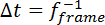, the area-average velocity, where refers to interrogation area . In the current experiments, each interrogation area consisted of n x n = 32 x 32 pixels ; the total number of interrogation areas subdividing each 210 mm x 160 mm FOV was thus 47 x 35, corresponding to 1504 x 1128 pixels.

5. Process Vibrational Data

NOTE: Step 5 may be done simultaneously with Step 4 if different computer systems or analysis software is used.

1. Open data analysis software and by using the "load()" function to bring in the accelerometer data that was acquired when the vibratory bowl was empty (Step 1.2.2). Do a fast fourier transform of the data using the "fft()" function. Create a figure of the data using the "plot" function. Repeat with the data that was acquired when the vibratory bowl had media present (Step 1.2.5).
   NOTE: This process/data analysis function is available for multiple types of data analysis software and is written as a complete program by the researcher.
   1. In order to study molecular hydrodynamic processes, a number of data processing operations are generally required. See the Representative Results and Discussion sections below for outlines of the main processing procedures; see Keanini, et al. (2017)¹² for details on how measured PIV data can be used to extract dynamical information on molecular hydrodynamic systems.

Results

In presenting representative results, we refer to continuum-time-scale processes as those observed and predicted over time-scales, that are long relative to the characteristic grain collision time scale,

Discussion

In order to use vibrated grain piles as macroscopic analogs for investigating molecular hydrodynamic processes, an experimentalist must, on one hand, learn and use four basic measurements, and on the other, master a few basic elements of equilibrium and non-equilibrium statistical mechanics. Focusing first on experimental measurements, these include: i) measurement of individual grain dynamics through measurement of the single-particle velocity autocorrelation function, ii) measurement of time-average/long-time-scale sur...

Materials

List of materials used in this article

Name	Company	Catalog Number	Comments
Vibratory Polishing Bowl	Raytech	AV-75
Flow Meter	Peristaltic Pumps	913 Mity Flex
Scale	Pelouze	4040
Triaxial Accelerometer	PCB Piezotronics	PCB 356B11	Accelerometer with Sensor Signal Conditioner
Data Acquisition Computer	IBM	Thinkpad	Used with high speed camera
High Speed Camera	Redlake	Motionxtra HG-XR
Zoom Lens	Tamron	Model A18	18-250mm F/3.5-6.3
High intensity Light	ARRI	EB 400/575 D
Data Processing Computer	Dell	Dell Precision Tower 7910
PIV Software	Dantec Dynamics	Dynamic Studio 2013	version 3.41.38
Data Acquisition Hardware	National Instruments	SCXI	SCXI-1000 Chasis with SCXI 1100 Card and SCXI 1303 Adapter
Data Acquisition Software	National Instruments	LabVIEW 2012
Data Processing Software	MATHWORKS	MATLAB
Polishing Media	Rosler	RSG 10/10S	Multiple media types used (mixed, spherical, triangular)
Polishing Solution	Rosler	FC KFL (3%)	3% soap solution with water
Ruled Scale	Swiss Precision Instruments	13-911-3
Graduated Cylinder	Global Scientific	601082