Imaging techniques that reflect dynamic bone turnover may aid in characterizing a wide range of bone pathologies. We present detailed methodologies for performing and analyzing dynamic [18F]-NaF-PET-MRI data in a patient with facetogenic low back pain using the lumbar facet joints as a prototypical region of interest.
A subscription to JoVE is required to view this content. Sign in or start your free trial.
Method Article
Quantitative [18F]-Naf-PET-MRI Analysis for the Evaluation of Dynamic Bone Turnover in a Patient with Facetogenic Low Back Pain
In This Article
Summary
Abstract
Imaging techniques that reflect dynamic bone turnover may aid in characterizing a wide range of bone pathologies. Bone is a dynamic tissue undergoing continuous remodeling with the competing activity of osteoblasts, which produce the new bone matrix, and osteoclasts, whose function is to eliminate mineralized bone. [18F]-NaF is a positron emission tomography (PET) radiotracer that enables visualization of bone metabolism. [18F]-NaF is chemically absorbed into hydroxyapatite in the bone matrix by osteoblasts and can thus noninvasively detect osteoblastic activity, which is occult to conventional imaging techniques. Kinetic modeling of dynamic [18F]-NaF-PET data provides detailed quantitative measures of bone metabolism. Conventional semi-quantitative PET data, which utilizes standardized uptake values (SUVs) as a measure of radiotracer activity, is referred to as a static technique due to its snapshot of tracer uptake in time. Kinetic modeling, however, utilizes dynamic image data where tracer levels are continuously acquired providing tracer uptake temporal resolution. From the kinetic modeling of dynamic data, quantitative values like blood flow and metabolic rate (i.e., potentially informative metrics of tracer dynamics) can be extracted, all with respect to the measured activity in the image data. When combined with dual modality PET-MRI, region-specific kinetic data can be correlated with anatomically registered high-resolution structural and pathologic information afforded by MRI. The goal of this methodological manuscript is to outline detailed techniques for performing and analyzing dynamic [18F]-NaF-PET-MRI data. The lumbar facet joint is a common site of degenerative arthritis disease and a common cause for axial low back pain. Recent studies suggest [18F]-NaF-PET may serve as a useful biomarker of painful facetogenic disease. The human lumbar facet joint will, therefore, be used as a prototypical region of interest for dynamic [18F]-NaF-PET-MRI analysis in this manuscript.
Introduction
Standard clinical imaging techniques of bone pathology are primarily limited to characterizing structural changes, which can be nonspecific. For example, asymptomatic morphologic abnormalities related to the normal aging may be indistinguishable from degenerative alterations which are responsible for severe pain and disability1. Bone is a dynamic tissue undergoing continuous remodeling with the competing activity of osteoblasts, which produce the new bone matrix, and osteoclasts, whose function is to eliminate mineralized bone2. [18F]-NaF is a positron emission tomography (PET) radiotracer that enables visualization of bone tissue metabolism. [18F]-NaF is chemically absorbed into hydroxyapatite in the bone matrix by osteoblasts and can thus noninvasively detect osteoblastic activity, thereby detecting a metabolic process which is occult to conventional imaging techniques. As a result, [18F]-NaF has been used for characterizing bone pathology in an increasing number of bone disorders including neoplasms, inflammatory, and degenerative disease of the bone and joints3,4,5.
PET data is most commonly analyzed in a semi-quantitative fashion, which can be readily performed in routine clinical practice with standardized uptake values (SUVs). As a metric, SUVs are useful to clinicians as they represent tissue uptake relative to the rest of the body6. Values from subsequent scans may be used to observe changes in uptake as a result of treatment or disease progression. The numerical nature of SUVs also aids in comparison between patients and between successive scans in the same patient. The algorithm used to calculate SUVs, Equation 1, makes the assumption that the tracer is equally distributed throughout the body and that the lean body mass accurately represents whole body volume. As such, SUVs are a semi-quantitative measurement. For a given region of interest (ROI), SUVmax (the maximum SUV value within a ROI), and SUVmean (the mean of all sampled SUVs within an ROI) are commonly used SUV metrics in clinical practice6.
Kinetic modeling of dynamic PET data can also be performed for more detailed quantitative analysis. While SUV data acquisition is static, kinetic modeling utilizes dynamic image data where tracer levels are continuously acquired providing a temporal dimension. From the more complex kinetic modeling of dynamic data, quantitative values and informative metrics of tracer dynamics can be extracted with respect to the measured activity in the image data. A sample two-tissue compartment model employed for dynamic kinetic modeling is shown in Figure 17. Cp is the concentration of tracer in the blood plasma while Ce and Ct represent the concentration in the unbound interstitial space and bound tracer in the target bone matrix respectively. K1, k2, k3, k4, are 4 rate parameters that describe the kinetic model for tracer wash in/out and binding. K1 describes the tracer taken up from arterial plasma into interstitial space (Ct), k2 describes the fraction of tracer that diffuses back from the interstitial space to plasma, k3 describes the tracer that moves from interstitial (Ce) space to bone (Ct), and k4 describes the tracer that moves from bone (Ct) back to the interstitial space (Ce).

Figure 1. A sample two-tissue compartment model for dynamic kinetic modeling. Cp is the tracer concentration in the blood plasma compartment, Ce free and non-specifically bound tracer concentration in tissue, and Ct specifically bound tracer concentration in the tissue. Please click here to view a larger version of this figure.
The Patlak kinetic model produces Ki_Patlak as a measure of radiotracer influx rate (mL/ccm/min, cubic cm = ccm) from the blood pool into the bone matrix. The tracer influx rate from the blood pool to the bone matrix can then be calculated using Equation 2 and Equation 3 for Ki_Patlak and Ki_NonLinear respectively. Ki_Patlak and Ki_NonLinear are the rates at which [18F]-NaF leaves the arterial blood pool and irreversibly binds to a subsite bone matrix, using the two models respectively. A difference between the Patlak and non-linear kinetic model is in their utilization of the dynamic data. The Patlak model requires equilibrium to be met and then calculates the influx rate from the established linear slope. The Patlak kinetic model produces Ki_Patlak influx rates, by using a 24-minute time to equilibration of the plasma pool, Cp, to the unbound pool, Cu. The 24-minute time can change depending on the time found for all subsites to reach equilibration with the plasma pool in the sample. The more computationally rigorous non-linear model uses the entirety of the temporal data to fit a curve.
The goal of this methodological manuscript is to outline detailed techniques for performing dynamic [18F]-NaF-PET-MRI. The lumbar facet joint is a common site of degenerative arthritis disease and a common cause for axial low back pain8. Recent studies suggest [18F]-NaF-PET-MRI may serve as a useful biomarker of painful facetogenic disease9. The human lumbar facet joints from a single patient with facetogenic low back pain will thus be analyzed as a prototypical ROI for dynamic [18F]-NaF-PET-MRI analysis.
Access restricted. Please log in or start a trial to view this content.
Protocol
This prospective feasibility study recruited patients after obtaining Human Study IRB approval and complying with HIPAA regulations.
1. Phantom
- Fill a hollow cylindrical phantom with an insert that has hollow cylinders with a range of diameters (5 - 38 mm) with 185 MBq of [18F]-NaF.
- Generate an attenuation map of the phantom using CT or a template that was generated previously for this phantom.
- Place the phantom into the center of PET/MR and acquire PET data for 5-10 min recording the resultant image using the imaging console.
- Reconstruct using the imaging console with the CT-based attenuation map using an algorithm that matches with the same reconstruction algorithm to be used for imaging human subjects.
- Calculate the mean activity in each cylinder (left and right) of equal size for all sizes using freeware AMIDE.
- Tabulate the mean activity versus cylinder size.
- Calculate the partial volume errors (PVE) by dividing the mean activity of each cylinder by the reference cylinder mean activity.
- Plot the PVE by the size of the cylinder.
- Use the linear equation between two-cylinder sizes when correcting for PVE in the patient data.
2. Patient Preparation
- Before recruiting patients, obtain any necessary Human Study IRB approval and comply with HIPPA regulations.
- Establish appropriate inclusion and exclusion criteria for the study of interest.
- Inclusion criteria were as follows: adults, at least 18 years old with the capacity for informed consent; a reported history of axial non-radicular low back pain; recommended by the spine interventional radiologists.
- Exclusion criteria were as follows: the history of fracture or tumor of the spine; women who are pregnant or breast-feeding; contraindications to having MRI or administration of tracer or contrast; prior lumbar surgery or instrumentation.
- Gather patient’s written informed consent, approved by the Committee on Human Research.
- Obtain any relevant clinical exam and/or patient survey data pertinent to your study of interest.
- Have subject change into the gown, establish IV access, administer pregnancy test if the patient is female and of child-bearing age, check creatinine/GFR for the safe use of contrast, and retrieve [18F]-NaF dose. Coach the patient on the importance of remaining still throughout the duration of the exam.
- Position patient supine and feet first in the PET/MRI.
3. Imaging Protocol
- Use a 3.0 T PET/MRI scanner for simultaneous PET and MR image acquisition.
- Use the posterior array central molecular imaging array coil for the MR imaging.
- Ensure the FOV of both MR and PET imaging modalities is centered to cover the lower spine region from T12 to S3.
- The Clinical MRI sequences for the lumbar spine protocol includes: Sagittal T1 (repetition time/echo time (TR/TE) = 510/8.6 ms, in-plane resolution = 0.75mm, through-plane resolution = 4mm), Sagittal T2 fat saturated (FS) (TR/TE = 4208/86.2 ms, in-plane resolution = 0.75mm, through-plane resolution = 4mm) Axial T2 fast relaxation fast spin echo (FRFSE) with and without fat saturation (TR/TE = 750/9.2 ms, in-plane resolution = 0.7mm, through-plane resolution = 4mm), Axial T1 fast spin echo (FSE) Pre Gadolinium (TR/TE = 575/8.9 ms, in-plane resolution = 0.65mm, through-plane resolution = 4mm), Axial T1 FSE Post Gadolinium (TR/TE = 562/8.6 ms, in-plane resolution = 0.65mm, through-plane resolution = 4mm).
- Inject 0.1 mm/kg of gadobutrol (1M Gadavist) contrast into the patient’s antecubital fossa IV directly before acquiring the MRI sequences requiring it.
- Prior to the dynamic PET scan inject the radioactive dose of [18F]-NaF into the patient at a concentration of 2.96 MBq/kg of [18F]-NaF.
- Perform a 60 min of dynamic PET scan using 3 separate temporal phases centered over the lower spine, T12 to S3.
- Acquire the first phase of the dynamic scan with 12 frames of 10 s each.
- Acquire the second phase of 4 frames of 30 s each.
- Acquire the last phase of 14 frames of 4 min each.
- Calculate MR attenuation correction (MRAC) for the lumbar spine region using the standard two-point Dixon method. The Dixon method segments the MR signals of fat and water into air, soft tissue, lung and fat (though not bone).
- Ensure PET data is co-registered to axial T2 fat saturated FRFSE images.
- Reconstruct the PET data on the console using the following parameters: 60 cm field of view (FOV), 3 mm post-filter, Standard Z-axis filter, 256 x 256 matrix, 28 subsets, and VPFX (Time of Flight - Ordered Subsets Expectation Maximization, TOF-OSEM) with 4 iterations.
- Ensure reconstruction includes post processing to correct for decay, attenuation, scatter, and dead time.
4. Image analysis
- Have blinded radiologist interpret the clinical MRI sequences.
- Evaluate fat-suppressed T2- weighted and fat suppressed T1-weighted post-contrast sequences for grading facet synovitis as previously described by Czervionke and Fenton10.
- Use the following facet grading is: MRI grade 0 = no abnormality of the facet joint, 1 = abnormal enhancement or T2 hyperintensity limited to joint capsule, 2 = abnormal extracapsular enhancement or T2 hyperintensity involving < 50% of FJ perimeter, 3 = abnormal extracapsular enhancement or T2 hyperintensity involving >50% of FJ perimeter, and 4 = grade 3 with extension of edema into the neuroforamen, ligementum flavum, pedicle, transverse process, or vertebral body. As explained in the ref: Czervionke LF, Fenton DS. Fat-saturated MR imaging in the detection of inflammatory facet arthropathy (facet synovitis) in the lumbar spine.10
5. Data analysis
- Transfer PET and MRI images to a dedicated workstation equipped to analyze dynamic PET data such as the software PMOD. Analyze the facet joints of the lumbar spine from L1-L2 to L5-S1.
- Locate regions that will be evaluated for [18F]-NaF uptake measurements: bilateral facet joints at each level. Select volumes of interest (VOI) using anatomic T2 MR images and then transfer to the PET images.
- Identify the center point of each lumbar facet joint by visually triangulating with sagittal and axial plane T2 MR images and recording the slice number of the approximate center.
- With the patient data open in the View tab, click the VOI button from the sidebar and select SPHERE (Object).
- Within the Predefined window that pops up, type in 7.5 mm as the radius and click Create New VOI.
- Place a spherical VOI (7.5 mm diameter) in the center of each facet joint by left clicking on the facet. Adjust the sphere by left clicking and dragging until visually centered on the facet.
- Repeat as necessary for all facets of interest by clicking Create New VOI and performing step 5.5
- Place a spherical VOI (5 mm diameter) in the right iliac crest in the central marrow cavity (to exclude cortex involvement) as a reference region. Click Create New VOI and left click in the marrow of right iliac.
- Position VOI so edges are within marrow entirely.
- Ensure VOI’s are placed similarly to the image showing vertebral body facet joint (FJ) VOIs in Figure 2 in that they encapsulate the center of the facet joint.
6. SUV Calculations and Kinetic Data
- To calculate the arterial input function place a cylindrical VOI covering two axial slices of the abdominal aorta. Ensure the diameter is equal to the aorta’s diameter.
- Right click on the Axial image, select data inspection.
- Measure the diameter of the abdominal aorta proximal to its bifurcation.
- Left click on the right side of the aortic wall and move the cursor to the left side of the aortic wall.
- Record the distance of the aortic wall diameter in the Data Inspector window. This will be used to calculate the partial volume correction (PVC) coefficient.
- Left click the VOI button from the sidebar, select CIRCLE (ROI).
- Create a Circle ROI with a specified radius of half of the previously measured diameter in Step 6.5
- Click Create New VOI and left click in the center of the aorta, reposition if necessary, to ensure circle approximates aortic wall position.
- Descend one slice in the axial plane and repeat steps 6.7-6.9, thereby, making a cylinder from the two circular ROI’s.
7. PET Partial Volume Correction
NOTE: Due to PVE the tracer activity is underestimated in relation to the size of the target. Therefore, steps are taken to correct for the PVE.
- Use the recovery coefficients that were derived earlier using the PET/CT phantom by plotting the size of the cylinder diameter versus the ratio of recovered activity to true activity.
- Apply the recovery coefficients to the image-based measurement over the descending aorta to create a partial-volume corrected arterial input.
- Substitute this partial-volume corrected arterial input into PMOD for use in kinetic modeling and accurate quantification of tracer kinetics.
8. SUV Calculations and Kinetic Data
Note: The algorithm used to calculate Standard Uptake Value (SUV), Equation 1, makes the assumption that the tracer is equally distributed throughout the body and that the lean body mass accurately represents whole body volume. Therefore, SUVs are referred to as a semi-quantitative measurement.
Equation 1: Standard Uptake Value

- Calculate the SUVmax, and SUVmean values for each subsite using the 60-minute time point.
Note: The two-tissue compartment model used for kinetic modeling is shown in Fig 1. Cp is the concentration of tracer in the blood plasma while Ce and Ct represent the concentration in the unbound interstitial space and bound tracer in the target bone matrix respectively. K1, k2, k3, k4, are 4 parameters that describe the kinetic model for tracer wash in/out and binding. - Use the two-tissue compartment irreversible for Patlak Linear model and Non-Linear regression models during kinetic analysis
Note: A two-tissue irreversible compartment model is used to calculate region-specific influx rate constants (in min-1) for [18F]-NaF11. - Ensure the time to equilibrium is set to 24 minutes when using the Patlak kinetic model
- Input k4 = 0 when using the nonlinear regression model to produce Ki_NonLinear influx rates.
- Calculate the tracer influx rate from the blood pool to the bone matrix using Equation 2 and Equation 3 for Ki_Patlak and Ki_NonLinear respectively. Ki_Patlak and Ki_NonLinear are the rates at which [18F]-NaF leaves the arterial blood pool and irreversibly binds to a subsite bone matrix, using the two models respectively.
- Equation 2: Patlak Graphical Kinetic Model
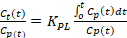 + Intercept
 - Equation 3: Nonlinear Regression Kinetic Model
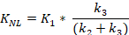
- Equation 2: Patlak Graphical Kinetic Model
9. Statistical Analysis
- Use a linear regression analysis to evaluate if [18F]-NaF Ki_Patlak influx rate was correlated to: SUVmean, SUVmax, Ki_NonLinear, and any clinical scoring grades specific to the study.
- Use two-tailed t-test and Pearson correlation to test for statistical significance in previous correlations.
Access restricted. Please log in or start a trial to view this content.
Results
18NaF-PET uptake values are measured in the bilateral facet joints at the L1-L2 through L5-S1 vertebral levels for a total of 10 ROIs in a single representative patient with axial low back pain. Representative [18F]-NaF-PET, axial T2 fat suppressed, and axial T1 post-contrast fat-suppressed MR images through the level of the L3-L4 facet joints are shown in Figure 2. The Ki_Patlak, SUVmean, SUVmax, and MRI facet arthropathy grade for eac...
Access restricted. Please log in or start a trial to view this content.
Discussion
In this methodological manuscript, we have provided background on the potential utility of dynamic [18F]-NaF-PET-MRI for evaluating a wide range of bone pathologies and have outlined the techniques for dynamic [18F]-NaF-PET-MRI image acquisition and analysis using the human lumbar facet joints as prototypical regions of interest. Dual modality PET-MRI allows for acquisition of dynamic PET data over a time period similar to that required for MR data acquisition alone, thus maximizing the overlap of s...
Access restricted. Please log in or start a trial to view this content.
Disclosures
The authors have nothing to disclose
Acknowledgements
Research support was provided by NIH P50AR060752 and GE Healthcare. We would like to acknowledge the support by Vahid Ravanfar.
Access restricted. Please log in or start a trial to view this content.
Materials
| Name | Company | Catalog Number | Comments |
|---|---|---|---|
| Gadolinium Contrast agent (Gadovist) | Bayer | na | 1.0mmol/ml solution for IV injection. |
| [18F]-NaF Radiotracer | na | na | 2.96 MBq/kg |
| GE Signa PET-MRI Scanner | General Electric | na | 3.0Tesla 60cm Bore PET-MRI scanner |
| PMOD Kinetic Modeling Software | PMOD Technologies, LLC | na | Version 3.8 |
References
- Brinjikji, W., et al. Systematic literature review of imaging features of spinal degeneration in asymptomatic populations. AJNR American Journal of Neuroradiology. 36 (4), 811-816 (2015).
- Binder, D. S., Nampiaparampil, D. E. The provocative lumbar facet joint. Current Reviews in Musculoskeletal Medicine. 2 (1), 15-24 (2009).
- Spick, C., et al. Detection of Bone Metastases Using 11C-Acetate PET in Patients with Prostate Cancer with Biochemical Recurrence. Anticancer Research. 35 (12), 6787-6791 (2015).
- Brans, B., et al. Assessment of bone graft incorporation by 18 F-fluoride positron-emission tomography/computed tomography in patients with persisting symptoms after posterior lumbar interbody fusion. EJNMMI Research. 2 (1), 42(2012).
- Jadvar, H., et al. Prospective evaluation of 18F-NaF and 18F-FDG PET/CT in detection of occult metastatic disease in biochemical recurrence of prostate cancer. Clinical Nuclear Medicine. 37 (7), 637-643 (2012).
- Kinahan, P. E., Fletcher, J. W. Positron emission tomography-computed tomography standardized uptake values in clinical practice and assessing response to therapy. Seminars in Ultrasound, CT, and MR. 31 (6), 496-505 (2010).
- Hawkins, R. A., et al. Evaluation of the skeletal kinetics of fluorine-18-fluoride ion with PET. Journal of Nuclear Medicine: Official Publication, Society of Nuclear Medicine. 33 (5), 633-642 (1992).
- Hancock, M. J., et al. Systematic review of tests to identify the disc, SIJ or facet joint as the source of low back pain. European Spine Journal: Official Publication of the European Spine Society, the European Spinal Deformity Society, and the European Section of the Cervical Spine Research Society. 16 (10), 1539-1550 (2007).
- Jenkins, N. W., et al. [18)F]-Sodium Fluoride PET MR-Based Localization and Quantification of Bone Turnover as a Biomarker for Facet Joint-Induced Disability. AJNR American Journal of Neuroradiology. 38 (10), 2028-2031 (2017).
- Czervionke, L. F., Fenton, D. S. Fat-saturated MR imaging in the detection of inflammatory facet arthropathy (facet synovitis) in the lumbar spine. Pain Medicine. 9 (4), 400-406 (2008).
- Phelps, M. E., et al. Tomographic measurement of local cerebral glucose metabolic rate in humans with (F-18)2-fluoro-2-deoxy-D-glucose: validation of method. Annals of Neurology. 6 (5), 371-388 (1979).
- Brenner, W., et al. Comparison of different quantitative approaches to 18F-fluoride PET scans. Journal of Nuclear Medicine: Official Publication, Society of Nuclear Medicine. 45 (9), 1493-1500 (2004).
- Schellinger, D., et al. Facet joint disorders and their role in the production of back pain and sciatica. Radiographics: A Review Publication of the Radiological Society of North America, Inc. 7 (5), 923-944 (1987).
- Schett, G. Joint remodelling in inflammatory disease. Annals of the Rheumatic Diseases. 66, Suppl 3 42-44 (2007).
- Baum, R., Gravallese, E. M. Impact of inflammation on the osteoblast in rheumatic diseases. Current Osteoporosis Reports. 12 (1), 9-16 (2014).
Access restricted. Please log in or start a trial to view this content.
Reprints and Permissions
![Quantitative [18F]-Naf-PET-MRI Analysis for the Evaluation of Dynamic Bone Turnover in a Patient with Facetogenic Low Back Pain](/_next/image?url=https%3A%2F%2Fcloudfront.jove.com%2FCDNSource%2Fteasers%2F58491.jpg&w=3840&q=75)