Generating Strictly Controlled Stimuli for Figure Recognition Experiments

Summary

This protocol describes a method for an experiment that examines whether specific graph and non-graph properties (features) are relevant to the recognition of figures. The method uses a database that stores various feature values of respective figures called (6 point, n line) figures.

Abstract

This protocol introduces a method for generating strictly controlled and objectively defined stimuli for figure recognition experiments. A (6, n) figure consists of n line segments that are spanned between n pairs of points located at the vertices of an invisible regular hexagon. The structural properties (graph invariants) and superficial features (non-graph invariants) of each (6, n) figure with n values ranging from 1 to 6 are calculated and stored in a database. Using this database, experimenters can systematically extract appropriate figures depending on the purpose of the experiment. Furthermore, if the database does not contain necessary information, new feature values can sometimes be calculated ad hoc from the formation of a specific (6, n) figure. Let us call a mirror-reflected pair of figures an axisymmetric (Ax) pair. An Ax pair of figures is known to be more difficult to discriminate than a non-identical pair in the decision of whether the shapes of a given pair are rotated-to-be-identical (Idr). The purpose of the present experiment is to examine whether the sameness of line lengths between two figures in a pair causes the discrimination of the pair to be as difficult as that of an Ax pair. Mutually isomorphic figures share common structural properties despite differences in shape. Ax pairs and Idr pairs are special cases of isomorphic pairs. Furthermore, an Ax pair and Idr pair share most of the superficial feature values, except the relative direction from one location to another location across an axis of symmetry is opposite for an Ax pair. Three types of mutually isomorphic (6, 4) figure pairs were generated: Idr; Ax; and non-identical, non-axisymmetric, isomorphic (Nd) pairs. Nd pairs were further classified into three subcategories according to the superficial feature values of the degree of line length differences.

Introduction

This paper describes a method for generating strictly controlled and objectively defined stimulus figures for studies on the recognition of random figures. The stimuli are called (6 point, n line) or (6, n) figures. A (6, n) figure consists of n line segments that are spanned between n pairs of points located at the vertices of an invisible regular hexagon. Figure 1 shows an example of a (6, 4) figure that is specified by four pairs of labels for the vertices of an invisible regular hexagon. The labels designate the line segments of the figure (see Figure 1). Let us call this specification of figures a line specification format.

Formerly, the author calculated the graph theoretical structural properties of (6, n) figures (called invariant features, or more specifically graph invariants¹) and non-invariant properties (called superficial features) for figures with n = 1 to 6 and stored the feature values in a database. Invariant features reflect the structural (more precisely, topological) properties and superficial features reflect the non-topological and mostly metric properties of a given figure.

A record number in the database uniquely identifies a figure in the line specification format. Therefore, an exhaustive search for specific values of invariant and/or superficial feature values in the database enables the retrieval of the record numbers for the figures that satisfy the conditions from the total set of (6, n) figures. The retrieved figures can serve as the stimuli for an experiment. Each record in the database contains variables that include the isomorphic set to which the figure belongs; various graph invariants, such as the number of cycles, circumference, point covering number, number of critical points, radius, number of central points, number of components, maximum degree, number of maximum degree points, number of isolated points, and number of endpoints; non-graph feature values, such as the number of intersections, and jaggedness of the contours defined by vertices and intersections; and superficial feature values, such as locations of the invariant features and (in the case in which there are plural locations) the directions formed by plural locations. For example, a cycle indicates a closed sequence of line segments, a degree of a point is the number of line segments incident with that point, an isolated point is a point with a degree of 0, and an endpoint is a point with a degree of 1. Using the invariant feature values of the database, all (6, n) figures from n = 1 to 6 can be sorted into the numbers of isomorphic sets shown in Appendix 1¹. See Figure 2 for an example of the stored information in each record.

Note that the figures that belong to each isomorphic set are topologically equivalent despite differences in shape. Several studies have claimed that topological structures are perceived prior to more specific properties of given figures^2,3,4,5. By systematically changing stimulus figures, the author claimed that detections and comparisons of invariant features precede the detections and comparisons of superficial features⁶. The present experiment is an attempt to clarify whether the superficial feature of line length is critical in the recognition of figure pairs under the condition that invariant feature values are all equivalent between the figure pairs (i.e., mutually isomorphic).

The types of stimulus figures that are used in experiments is critically important to figure recognition research. There are two types of stimulus figures: those that are randomly generated and those that are generated ad hoc for the purpose of a study. To reduce confounds associated with factors not under experimental control, the use of randomly generated figures is generally considered to be more appropriate. There are several types of random figures, for example, random histograms⁷ and random matrices⁸, but the most frequently used random figures in visual recognition research in psychology are random polygons⁹. A general rule for making random polygons is to connect randomly distributed locations of n points in a square area with line segments in such a manner that the perimeter of the line segment is mostly convex and then color inside the perimeter. A frequently used objective index for random polygons is the number of flections of the perimeter of a polygon, which represents the complexity of the figure^10,11,12. As the inside of the figure is colored in, structural properties regarding its perimeter are limited to the number of flections. Additionally, with the exception of the number of flections, no information is given about either the entire set of random polygons or the relationship between distinct random polygons.

The figures in axisymmetric (Ax) pairs of figures are known to be more difficult to discriminate than non-identical pairs in a task to decide whether a given pair of figures is rotated-to-be-identical (Idr)^13,14,15. The two figures in an Idr pair and those in an Ax pair are mutually isomorphic and have corresponding line segments that are the same length. However, whether sameness of line lengths between the two figures in a pair increases the difficulty of discrimination of a non-identical pair compared with that of an Ax pair is unclear. In this experiment, participant discrimination performance was compared between Ax pairs and non-identical, non-axisymmetric (Nd) pairs. The differences in line lengths were experimentally controlled between the two figures. Because of the precedence of detecting invariant feature value differences prior to superficial feature value differences during figure recognition⁵, the Nd figure pairs were set to be mutually isomorphic so that line length differences would not be confounded with invariant feature value differences.

Experiment 1 in the author-used (6, 5) figure pairs to examine the hypothesis that the lack of line length differences influenced the level of difficulty of discrimination of the figures in Ax pairs¹⁵. The results demonstrated that the latencies were shorter for Nd 0 (viz., no difference in total line length between paired figures) pairs compared with those for Ax pairs, which indicated that the hypothesis was unsupportable. It was argued that superficial feature value differences not under experimental control are more likely to be present in complex figures, and participants might make use of these. Interestingly, several studies have claimed that the presence of a cycle is preattentively detected^16,17. By contrast, Julesz claimed that the presence of an endpoint was detected at an early stage of the segregation of figures from the background¹⁸.

To address this, simpler (6, 4) figure pairs were chosen to examine the hypothesis. Out of nine isomorphic sets of (6, 4) figures, the figures that belonged to two isomorphic sets were used as stimuli. Both sets of figures shared easily detectable invariant features of (an) endpoint(s) and a cycle (i.e., a triangle) in common. See the example figures of nine isomorphic sets in Figure 3. Additionally, see the column of p = 6 and q = 4 in Appendix 1¹.

Three basic pair types were generated: Idr, Ax, and Nd pairs. The total line length of a cycle (more specifically, a triangle) was equalized between the two figures in each pair for all pair types. Using this constraint, respective triangles of a figure pair became either mutually identical or Ax in shape. Nd pairs were further subcategorized according to differences in the lengths of endlines between the two figures in each pair, with the unit of length set as the side of an invisible regular hexagon. This yielded Nd 0, Nd 0.27, Nd 0.73, and Nd 1 pairs (i.e., the line length differences ranged from 0 to 1). As the presence of an intersection of line segments is known to be preattentively detected¹⁹, figures with intersecting line segments were excluded from the stimuli. See the examples of Idr, Ax, Nd 0, Nd 0.73, and Nd 1 pairs in Figure 4. To avoid the biased expectations of the participants, the number of Idr (‘same’) pairs was set to be the same as the sum of Ax (‘different’) and Nd (‘different’) pairs.

Protocol

The experiment was approved by the Hakuoh University Ethics Committee, Japan.

1. Experimental Setup

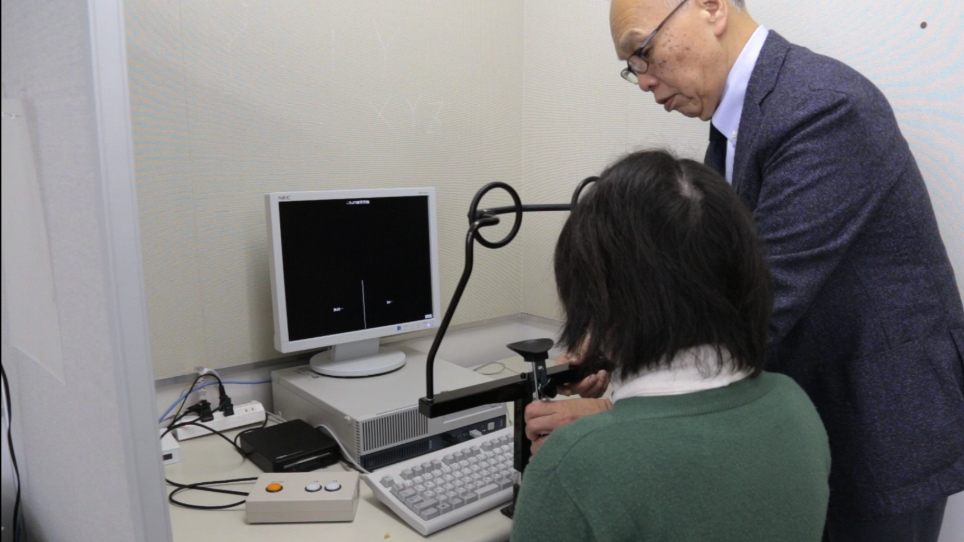
NOTE: The experimental environment consists of an LCD monitor and a response button box connected to a computer (PC for experiments). Each participant decides whether a presented pair of figures is the ‘same’ or ‘different’ by pressing one of the two buttons on a response box. There are three buttons on the box labeled ‘Enter’, ‘F6’, and ‘F5’ from left to right. By pressing the Enter button, the current screen proceeds to the next screen. The F6 button is for responses using the index finger and the F5 button is for responses using the middle finger of the participant’s right hand. The generation of figure pairs is done on a different computer (PC for stimulus preparation). This setup enables the examination of various hypotheses that concern the criticality of a certain feature in the recognition of figures in a fairly objective manner.

1. Insert a floppy disk into the floppy disk unit connected to the PC for stimulus preparation. Start the pair generation program on the PC for stimulus preparation.
2. Input a random number, using the keyboard, as an initial value to the random number generation function used in the program. Input either 1 or 2 using the keyboard as a digital specifier.
   NOTE: Digital specifier = 1 designates the index finger to ‘same’ decisions and the middle finger to ‘different’ decisions (digital state 1) in the first block of trials and vice versa (digital state 2) in the second block. Digital specifier = 2 designates digital state 2 in the first block and digital state 1 in the second block. This procedure counterbalances the speed of response by different fingers.

2. Instructions within the pair generation program

1. Open a stimulus set file (PRBLM2.DAT) as a new file on the floppy disk unit. Additionally, open the database file of (6, 4) figures on the main unit.
2. Sequentially examine each record of the database file from record number 1 to 1,365 to determine whether the record that has the value of the variable 28 (i.e., number of intersections of line segments, see Figure 2) is 0.
   NOTE: For the total numbers of (6, n) figures, see Corollary 15.1 (a)¹.
   1. If the value is not-0, discard the record and go to the next record, else examine whether the value of variable 1 (i.e., isomorphic set) is either 2 or 5.
   2. If the value is neither 2 nor 5, discard the record and go to the next record, else accumulate the record number as a candidate figure in an isomorphic 2 pool or an isomorphic 5 pool.
   3. Exhaustively combine each record with other records, including itself, of candidate figures that belong to the isomorphic 2 pool.
   4. Convert each pair of record numbers into their line specification formats in all candidate pairs.
   5. Examine whether a figure is paired with itself, and if it is, classify the pair as an Idr pair with a tag that indicates its angular distance 0° and accumulate it in a pool of Idr pairs.
   6. Else, add an integer from 1 to 5 to each vertex label number in the line specification format of one figure with modulo 6 residues. If the value is 0, convert it to 6. Then, standardize the format. Then, compare the standardized format of the figure with the line specification format of the other figure in the pair.
      NOTE: A line specification format of a (6, 4) figure consists of four sequences of pairs of point labels. It is expressed in accordance with the left label that is always smaller than the right label inside a pair, and the left label of a previous pair that is always smaller than or equal to the left label of the following pairs.
   7. If the two formats match with integer i, classify the pair as an Idr pair with a tag of its angular distance I (i.e., unit of 60° counterclockwise) and accumulate it in the pool of Idr pairs.
   8. Else, sequentially examine whether the pair is an Ax pair with one of the axes of symmetry being 0°, 30°, 60°, 90°, 120°, or 150° counterclockwise from the rightward horizontal.
      NOTE: The Ax transformation of a figure about an axis of symmetry 0° permutes point labels 1 for 6, 2 for 5, 3 for 4, and vice versa; about 30°, 1 for 1, 2 for 6, 3 for 5, 4 for 4, and vice versa; about 60°, 1 for 2, 3 for 6, 4 for 5, and vice versa; about 90°, 1 for 3, 2 for 2, 4 for 6, 5 for 5, and vice versa; about 120°, 1 for 4, 2 for 3, 5 for 6, and vice versa; and about 150°, 1 for 5, 2 for 4, 3 for 3, 6 for 6, and vice versa (Figure 5).
   9. If the line specification format of one figure after the Ax transformation about the axis of symmetry j° matches the format of the other figure in the pair, then classify the pair as an Ax pair with a tag of the axis of symmetry j° and accumulate it in a pool of Ax pairs.
   10. Else, classify the pair as an Nd pair. Then, calculate the numbers of incident lines at respective vertices in the line specification formats of the two figures of an Nd pair (Figure 6).
   11. If the number of incident lines is one at either end of a line segment of a figure, determine the segment as an endline of a figure. Then, determine the three remaining line segments as those constituting a cycle (i.e., a triangle).
   12. Calculate the total line lengths of the cycles of two figures of an Nd pair. If the total lengths of the cycles between the two figures differ, discard the pairs.
   13. Else, calculate the difference between line lengths of the endlines between two figures. If the length difference is 0, classify the pair as an Nd pair with a tag of 0 and accumulate it in the pool of Nd pairs.
   14. Else, if the length difference is 0.27, classify the pair as an Nd with a tag of 0.27 and accumulate it in the pool of Nd pairs.
   15. Else, if the length difference is 0.73, classify the pair as an Nd pair with a tag of 0.73 and accumulate it in the pool of Nd pairs.
   16. Else, classify the pair as an Nd pair with a tag of 1 and accumulate it with a tag of 1 in the pool of Nd pairs.
   17. Reiterate the protocol steps 2.2.3 to 2.2.16 for the candidate figures that belong to isomorphic set 5.
   18. Close the database file.
3. Preparation of a stimulus set for a participant
   1. Randomly sample three pairs from the Idr pool, two pairs from the Nd pool, and a pair from the Ax pool with tags as practice pairs.
   2. Concatenate Idr, Nd, and Ax practice pairs and randomize their presentation order for the first block of practice trials.
   3. Randomly sample 80 pairs from the Idr pool, 40 pairs from the Nd pool, and 40 pairs from the Ax pool with tags as test pairs.
   4. Concatenate Idr, Nd, and Ax test pairs and randomize their presentation order for the first block of test trials.
   5. Reiterate the protocol steps 2.3.1 to 2.3.4 for preparing practice and test trials in the second block of trials.
   6. Write a presentation number, digital state, pair type with a tag, number of line segments, and four pairs of vertex labels in the line specification format of the left figure and right figure of each trial to the floppy disk unit sequentially, and simultaneously echo these values on the screen.
   7. Reiterate step 2.3.6 from the first practice trial in the first block to the last test trials in the second block.
   8. Close the floppy disk unit.

3. Instruction by an experimenter and execution of an experiment by a participant

1. Ask each participant to provide written informed consent to participate in the experiment.
2. Instructions by an experimenter
   1. Instruct each participant to decide whether a presented pair of figures is identical in shape regardless of their orientations (‘Same’) or not (‘Different’) as quickly and accurately as possible and show example figure pairs.
3. Specifications before the experiment by an experimenter
   1. Start the stimulus presentation program on the PC for experiments.
   2. Click Identity decision task on the menu screen.
   3. Click Participant's information, then input name, sex, and age, and then click End of specification on the information screen.
   4. Click Read Stimulus data on the menu screen, click PRBLM2.DAT file in the floppy disk drive, and click OPEN on the file specification screen.
4. Execution of the experiment
   1. As an experimenter, seat a participant in front of the monitor and put his/her head on the chinrest and measure a distance 60 cm from the forehead to the monitor.
   2. As an experimenter, start an experiment by clicking Execution on the menu screen.
   3. As an experimenter, if the instruction screen shows the digital state 1, instruct a participant to press F6 key (response with the index finger) for ‘same’ decisions and to press F5 key (response with the middle finger) for ‘different’ decisions. If the instruction screen shows the digital state 2, instruct to press F6 for ‘different’ decisions and F5 for ‘same’ decisions.
   4. As a participant, after fully memorizing the digital state of the block, press Enter on the response box.
   5. As a participant, in response to the ‘Ready’ prompt on the screen, press Enter to start a trial.
   6. As a participant, upon the presentation of a pair of practice pairs on the stimulus screen, press the F6 or F5 key as soon as a decision is reached.
      NOTE: The six vertices of an invisible regular hexagon are stylized as small filled circles with diameters of 0.4 cm whose centers are shifted 0.2 cm outward from the locations of the vertices on a stimulus screen. The six vertices of a (6, 4) figure are projected in a 6.6 cm x 7.6 cm rectangular area. Two figures of a pair are located at horizontally parallel positions with a between-centers distance of 9.4 cm.
   7. (Previously) set up the stimulus presentation program to display ‘The decision was erroneous’ on the feedback message screen with a beep in a practice trial if a response is an error. If a response is correct, display ‘The decision was correct’ on the screen.
   8. As a participant, when confirming a feedback message, press Enter to proceed to the next ‘prompt’ screen.
   9. (As the stimulus presentation program), reiterate the steps 3.4.4 to 3.4.7 by the end of practice trials in the block.
   10. When all practice trials are complete, display ‘Start of the test trials’ on the screen.
   11. Reiterate the steps 3.4.4 to 3.4.5 at the end of test trials in a block.
       NOTE: The feedback messages are presented only during practice trials.
   12. Reiterate steps 3.4.3 to 3.4.8 to execute the practice and test trials in the second block.
   13. As the stimulus presentation program, save the data to a file on the floppy disk unit.
       NOTE: A participant’s data for each trial consists of a serial trial number, number of line segments, digital state, code of the pair type with a tag, code of the button pressed, correctness of a response, and latency in ms.

Representative Results

As Nd 0.27 pairs were found to only exist in the figures of isomorphic set 2, the subsequent analysis did not include the results for Nd 0.27 pairs. The hypothesis of the present study was that the sameness of line lengths between the two figures in Nd pairs would make them as difficult to discriminate as Ax figure pairs.

The results of the experiment are shown in Figure 7. Error rates were significantly different across the pair types, H = 23.8, p < 0.001. An ANOVA test showed that the latencies were different across the pair types, F (4, 48) = 12.3, p < 0.001. Scheffe’s tests showed that significant differences in latencies were not found between any pairs, except between Nd 0 and Nd 0.73, Nd 0 and Nd 1, and Nd 1 and Ax pairs. It is noteworthy that there was no difference in latency between Ax and Nd 0 pairs p ≈ 1.0.

The error rates and latency data both suggest that Nd 0.73 and Nd 1 pairs are easily discriminable compared with Ax pairs. However, the nearly absent difference in latency between Nd 0 pairs and Ax pairs strongly suggests that the sameness of line lengths caused Ax pairs to be more difficult to discriminate.

Figure 1. Example of a (6, 4) figure. The numbers near the filled circles indicate the labels of the points (i.e., vertices) of an invisible regular hexagon. The figure can be specified by four pairs of point labels (1-2, 1-3, 1-6, 3-6). Please click here to view a larger version of this figure.

Figure 2. Example of the content of the database of (6, 4) figures. Record number 3 (NR = 3) indicates the figure identifiable by the line specification format (1-2, 1-3, 1-4, 2-3). Variable (1) indicates the isomorphic set to which the figure belongs, (2) number of line segments, (3) number of cycles, (4) circumference, (17) maximum degree, (18) number of the points with the maximum degree, (21) number of isolated points, (24) number of endpoints, and (28) number of intersections of line segments. Please click here to view a larger version of this figure.

Figure 3. Examples of nine isomorphic sets of (6, 4) figures. The code numbers 1 to 9 do not indicate an order. Please click here to view a larger version of this figure.

Figure 4. Examples of pair types. (A) an Idr pair with an angular distance 120°, (B) Ax pair about the axis of symmetry 30° counterclockwise from the rightward horizontal, (C) Nd 0 pair, (D) Nd 0.73 pair, and (E) Nd 1 pair. Please click here to view a larger version of this figure.

Figure 5. Axes of symmetry that enable the permutation of specific pairs of point labels. Each line segment with a small number near its end is an axis of symmetry. Parenthesized numbers are point labels. This visualization enables the easy identification of pairs of points that are at equiangular distances from each axis. Please click here to view a larger version of this figure.

Figure 6. Illustrated example of line segments that are incident to the vertex points. Parenthesized large numbers indicate the point labels and smaller numbers indicate the number of line segments incident to the point. The line specification format of this figure is (1-4, 2-3, 2-4, 3-4), and the numbers of incident lines to the respective points are the summations of the appearance of the points in the format: 1 for point 1, 2 for 2, 2 for 3, 3 for 4, 0 for 5, and 0 for 6. As point 1 has 1 incident line, the point pair 1-4 is determined to be an endline and the remaining point pairs with a line incidence of more than 1 are taken to constitute a cycle. Please click here to view a larger version of this figure.

Figure 7. Mean latencies with standard errors of the means (hollow bars) and percent errors (grey bars) of the pair types. Idr denotes rotated-to-be-identical pairs; Nd denotes non-identical, non-axisymmetric, isomorphic pairs, where the number indicates the size of the difference in end line lengths between the two figures; and Ax denotes axisymmetric pairs. Please click here to view a larger version of this figure.

Discussion

The present method can be used to prepare a set of objectively definable stimulus figures for figure recognition experiments. The critical aspect of the method are the instructions within the pair generation program. Using a (6, n) database, the program can select appropriate candidate figures from the total (6, n) figures (protocol steps 2.2.1 and 2.2.2). Additionally, the program can sometimes calculate feature values of figures that are not stored in the database, as in the case of the calculation of the length of an end line (protocol step 2.2.13). If researchers wish to use a pair of figures as a unit of stimulus presentation, the program can exhaustively combine candidate figures to form pairs and sort them into geometrically justifiable categories, as explained in the categorization of Idr, Ax, and Nd pairs, in addition to in the subcategorization of Nd pairs (protocol steps 2.2.3‒2.2.16). If researchers are aware of possible confounding factors in advance, they can control these factors by adding or modifying instructions in the program, as in the cases of (a) using relatively simple (6, 4) figures pairs as stimuli (step 2.1); (b) avoiding having intersecting line segments in the figure (steps 2.2 and 2.2.1); and (c) equalizing the number of Idr pairs to the sum of the numbers of Ax and Nd pairs (step 2.3.3).

The pair generation program (file name: PMELCYLG2) was prepared ad hoc for the purpose of the present study. It is a partial modification of a previous program that includes routines for separating an end line from a triangle in a given figure, and then calculating the length of the end line. Taking this into account, the pair generation program has wide applicability because it introduces specific modifications to previous programs based on the current research question. Clearly, close debugging of the program is required before embarking on an experiment.

The applicability of the methods that use (6, n) figures is constrained by the nature of (6, n) figures per se and by the known properties (i.e., values of invariant and superficial features) of each (6, n) figure. A (6, n) figure consists of 6 points and n straight line segments that span n pairs of the points. The six points are assumed to be located coplanar and provide no depth information. Therefore, the methods are neither applicable to research questions that concern the recognition of concrete objects nor to those that do not concern figure features.

As already stated, randomly generated stimulus figures are generally more appropriate than those generated ad hoc for the specific purpose of a study. Unfortunately, the cases for using ad hoc figures exceed those for random figures. Even for the cases of using random polygons, the number of flections is a measure that lacks theoretical clarity and the total number of figures that have a number of flections equal to n is unknown. By contrast, invariant and superficial features used in the present method are supported by geometrical theories. Furthermore, the total sets of (6, n) figures with n = 1 to 6 are known and the figures that satisfy specific feature values are retrievable from the total set.

Concerning the end line in a figure of isomorphic set 2, its length and angle from the triangle were confounded. Regarding the figures that belonged to isomorphic set 5, the length of the detached end line was confounded with parallelism between the end line and a triangle. Such confusion could be resolved in the future by relaxing the condition that each line segment should be spanned between a pair of vertices of a regular hexagon.

Materials

Name	Company	Catalog Number	Comments
PC for stimulus preparation	DELL	Inspiron 15
External USB FD unit	Logitec	LFD-31UEF
Response button box	Takei Kiki	S-15068	custom item
PC for experiments	NEC	PC-37LB-N 15SN
LCD monitor	NEC	AS172-MC
Chin rest	Takei Kiki	T.K.K.930a
Pair generation program		PMELCYLG2	self-made
Database file		P4.DAT	self-made
Stimulus presentation program	Takei Kiki	Presentation/Response Device for (6, n) Figures	custom item

References

- Harary, F. Graph theory. , Addison-Wesley. Reading MA. (1969).
- Chen, L. Topological structure in visual perception. Science. 4573 (4573), (1982).
- Chen, L. Topological structure in the perception of apparent motion. Perception. 14 (2), 197-208 (1985).
- Hecht, H., Bader, H. Perceiving topological structure of 2-D patterns). Acta Psychol. 3 (3), 255 (1998).
- Todd, J. T., Chen, L., Norman, J. F. On the relative salience of Euclidean, affine, and topological structure for 3-D form discrimination. Perception. 3 (3), 273 (1998).
- Kanbe, F. On the generality of the topological theory of visual shape perception. Perception. 8 (8), 849-872 (2013).
- Fitts, P. M., Weinstein, M., Rappaport, M., Anderson, N., Leonard, A. Stimulus correlates of visual pattern recognition: A probability approach. J Exp Psychol. 1 (1), 1-11 (1956).
- Bethell-Fox, C. E., Shepard, R. N. Mental rotation: Effects of stimulus complexity and familiarity. J Exp Psychol Hum Percept Perform. 1 (1), 12-23 (1988).
- Attneave, F., Arnoult, M. D. The quantitative study of shape and pattern perception. Psychol Bull. 3 (3), 452-471 (1956).
- Cooper, L. A. Mental rotation of random two-dimensional shapes. Cogn Psychol. 7 (1), 20-43 (1975).
- Cooper, L. A., Podgorny, P. Mental transformations and visual comparison processes: Effects of complexity and similarity. J Exp Psychol Hum Percept Perform. 4 (4), 503-514 (1976).
- Folk, M. D., Luce, R. D. Effects of stimulus complexity on mental rotation rate of polygons. J Exp Psychol Hum Percept Perform. 3 (3), 395-404 (1987).
- Förster, B., Gebhardt, R., Lindlar, K., Siemann, M., Delius, J. D. Mental rotation effect: A function of elementary stimulus discriminability. Perception. 11 (11), 1301-1316 (1996).
- Kanbe, F. Can the comparisons of feature locations explain the difficulty in discriminating mirror-reflected pairs of geometrical figures from disoriented identical pairs. Symmetry. , 89-104 (2015).
- Kanbe, F. Are line lengths critical to the discrimination of axisymmetric pairs of figures from disoriented identical pairs. Jpn Psychol Res. 1 (1), 36-46 (2019).
- Treisman, A., Souther, J. Search asymmetry: A diagnostic for preattentive processing of separable features. J Exp Psychol Gen. 3 (3), 285-310 (1985).
- Kanbe, F. Which is more critical in identification of random figures, endpoints or closures. Jpn Psychol Res. 51 (4), 235-245 (2009).
- Julesz, B. Textons, the elements of texture perception, and their interactions. Nature. 290, 91-97 (1981).
- Wolfe, J. M., DiMase, J. S. Do intersections serve as basic features in visual search. Perception. 32 (6), 645-656 (2003).