This experimental protocol combined eye tracking and the assessment of presaccadic visual sensitivity in a dual task paradigm, consisting of a free choice saccade task and a visual discrimination task, to investigate the deployment of visual spatial attention before both, accurate and averaging saccades.
Method Article
Investigating the Deployment of Visual Attention Before Accurate and Averaging Saccades via Eye Tracking and Assessment of Visual Sensitivity
In This Article
Summary
Abstract
This experimental protocol was designed to investigate whether visual attention is obligatorily deployed at the endpoint of saccades. To this end, we recorded the eye position of human participants engaged in a saccade task via eye tracking and assessed visual orientation discrimination performance at various locations during saccade preparation. Importantly, instead of using a single saccade target paradigm for which the saccade endpoint typically coincides roughly with the target, this protocol comprised the presentation of two nearby saccade targets, leading to a distinct spatial dissociation between target locations and saccade endpoint on a substantial number of trials. The paradigm allowed us to compare presaccadic visual discrimination performance at the endpoint of accurate saccades (landing at one of the saccade targets) and of averaging saccades (landing at an intermediate location in between the two targets). We observed a selective enhancement of visual sensitivity at the endpoint of accurate saccades but not at the endpoint of averaging saccades. Rather, before the execution of averaging saccades, visual sensitivity was equally enhanced at both targets, suggesting that saccade averaging follows from unresolved attentional selection among the saccade targets. These results argue against a mandatory coupling between visual attention and saccade programming based on a direct measure of presaccadic visual sensitivity rather than saccadic reaction times, which have been used in other protocols to draw similar conclusions. While our protocol provides a useful framework to investigate the relationship between visual attention and saccadic eye movements at the behavioral level, it can also be combined with electrophysiological measures to extend insights at the neuronal level.
Introduction
Accumulated evidence argues for strong coupling between oculomotor and attentional control. The influential premotor theory of attention1,2 provides a particularly strict account regarding this coupling, suggesting that covert shifts of visual attention correspond to saccade programming without subsequent execution. Indeed, shared neuronal correlates of attentional and oculomotor control have been identified via functional magnetic resonance imaging (fMRI)3 and sub-threshold micro-stimulation of the Frontal Eye Fields (FEF) and the Superior Colliculi (SC) produces attentional benefits measured both behaviorally and electrophysiologically at the stimulated movement field position, even if no eye movements are induced4,5,6,7. Psychophysical experiments furthermore revealed that visual attention is consistently shifted towards the target of a saccade during oculomotor preparation8,9. However, dissociations at the neuronal level10,11,12 and observations that saccade preparation does not necessarily entail a corresponding shift of attention13,14,15,16 cast some doubt on an obligatory coupling between saccade programming and visual spatial attention.
Here, we revisited the nature of the coupling between attention and oculomotor programming at the behavioral level using a dual task which entailed a free choice saccade task and a visual discrimination task. Crucially, two saccade targets were presented at an angular distance of 30° on half of the trials, producing a distinct global effect17,18,19,20 associated with a substantial number of saccades landing in between the two targets (averaging saccades). Since we randomly presented a discrimination target shortly before saccade onset at one out of 24 equidistant locations (including the two saccade target locations, the location in between them and 21 control locations), we were able to assess and compare the presaccadic deployment of visual attention when saccade goal and saccade endpoint were either spatially associated (accurate saccades) or dissociated (averaging saccades).
To test whether visual attention is an obligatory consequence of oculomotor programming, and, therefore, always shifted towards the saccade endpoint, we analyzed visual sensitivity for all 24 locations as a function of the saccade landing direction. While accurate saccades were associated with a consistent presaccadic enhancement of visual sensitivity at their endpoint, we found no such enhancement at the endpoint of averaging saccades. This dissociation rules out an obligatorily coupling of visual attention to the executed oculomotor program at the behavioral level and suggests that attentional and oculomotor control are dissociable at some cortical or subcortical processing stage. Importantly, we observed an equal enhancement of visual sensitivity at the two saccade targets before averaging saccades, suggesting that the global effect arises from unresolved saccade target selection before saccade onset.
Protocol
This protocol was designed according to the ethical requirement specified by the Ludwig-Maximilians-Universität München and with the approval of the ethics board of the department.
1. Participants
- Recruit a sufficient number of naive participants with normal or corrected-to-normal vision and without neurological or psychiatric disorders. 10 participants are recommended based on similar, recent protocols21,22.
NOTE: Overall, we recruited 13 participants (aged 20-28, 7 females, 12 right-eye dominant, 1 author) from which 3 were excluded from final analysis since their orientation discrimination performance remained at chance level for all tested locations.
2. Experimental Setup
- Conduct the experiment in a quiet and dimly illuminated room under the supervision of an experienced experimenter familiar with eye tracking and all other experimental components.
- Prepare an experimental setup consisting of a computer, a cathode-ray tube (CRT) monitor, a standard keyboard, two loudspeakers, and an eye tracker (see Table of Materials).
- Sequence and control the experiment using an appropriate software (see Table of Materials). Write a script which can be run on the software to load and launch the experiment automatically for each participant (https://github.com/mszinte/CompAttExo). Ensure that the script encodes all necessary experimental parameters and implements stimulus presentation as well as behavioral and eye data collection.
- Display all visual stimuli on a CRT screen with a minimum vertical refresh rate of 120 Hz. Ensure the proper display of visual Gabors via gamma linearization of the experimental screen.
- Assess participants' evaluation of the discrimination target orientation (counterclockwise vs. clockwise) via the left and right arrow keys on a standard keyboard.
- Provide auditory feedback via loudspeakers upon incorrect manual responses.
3. Eye Tracking
- Record the gaze of participants' dominant eye at a sampling rate of at least 1 kHz throughout the entire experiment via an eye tracker.
- Ask the participant to sit down comfortably on a chair, place their chin on a chinrest, and lean their forehead against a bar to restrain head movement during the experiment. Individually adjust the height of the chair, the chinrest and the forehead bar such that participants' eyes align with the center of the experimental monitor.
- Individual Eye Tracker Calibration
- Before each experimental block (duration: approximately 10 min) and whenever necessary (e.g. after noticeable head movements and resulting shifts of the estimated fixation), run a calibration procedure to guarantee that participants' gaze can be accurately tracked within a radius of 1°.
NOTE: Here, we used a 13-point calibration procedure to get an accurate estimate of the characteristic light reflections (pupil and corneal reflection) of the tracked eye as a function of the gaze.- Ask the participant to follow a dot moving across different locations on the screen with their eyes to estimate their gaze position.
- Repeat the procedure with a dot rotation of 30° and compare the measured gaze position to the estimated gaze position to validate the initial calibration. The calibration can be considered accurate when the averaged difference between the estimated gaze position following the calibration stage and the measured gaze position in the validation stage is below 1°.
- Repeat the calibration procedure whenever the participant breaks fixation repetitively to guarantee high tracking accuracy throughout the experiment.
- Before each experimental block (duration: approximately 10 min) and whenever necessary (e.g. after noticeable head movements and resulting shifts of the estimated fixation), run a calibration procedure to guarantee that participants' gaze can be accurately tracked within a radius of 1°.
- During the experiment, monitor correct fixation at the screen center at the beginning of each trial. Only start a trial if the gaze stays within a radius of 2° around the central fixation target for at least 200 ms.
4. Instructions
- Provide participants with clear task instructions. Present the task instructions at least once at the beginning of each experimental session in the form of a written text, together with a visualization of the trial chronology. Encourage participants to carefully read through the instructions and to ask remaining questions to the experimenter.
NOTE: The instructions, as presented to the participants before each block, are shown in Figure 1.- Instruct the participant to fixate at the center of the screen at the beginning of each trial.
- Inform the participant that 24 flickering distractor streams will appear on the screen and that two of them will be cued by white frames, which will either be flashed shortly or remain on the screen until the trial end.
- Ask the participant to execute a saccade towards the center of one of the two cued distractor streams at free choice. Emphasize that participants should move their eyes as fast and as accurately as possible upon the onset of the cues.
- Inform the participant that, for a short duration during the trial, a tilted Gabor will be presented randomly at one of the 24 distractor streams.
- Ask the participant to manually report whether the tilted Gabor was rotated clockwise or counterclockwise relative to the vertical by pressing the right or left arrow on the keyboard, respectively. Explain that a sound will be played if the orientation of the tilted Gabor is being reported incorrectly.
5. Experimental Design, Stimuli, and Trial Chronology
- Ensure to partition the experiment into at least two experimental sessions on different days to guarantee participants' concentration across the entire duration of the experiment. Within an experimental session, prompt participants to take short breaks in between consecutive blocks.
NOTE: This experiment consisted of 24 blocks, each including 290 online correct trials (all trials without fixation breaks and with a saccade onset between 50 and 350 ms after the saccade targets onset; incorrect trials were repeated at the end of a block), amounting to a total duration of about 5 h. - Deliberately predefine stimulus features (color, luminance, and size), stimulus timing, and a viewing distance which ensures the desired angular stimulus size. While most features of the visual stimuli (e.g., size, luminance, and contrast) can be adjusted to account for specific experimental purposes based on piloting, precise stimulus timing is crucial to assess visual attention during the presaccadic interval.
- Stimuli and Trial Chronology
- Present all stimuli on a gray (~19.5 cd/m2) background in order to minimize visual and screen aftereffects.
NOTE: A visualization of the experimental procedure can be found in Figure 2. - Present a fixation target (FT) in the form of a black (~0 cd/m2) and white (~57 cd/m2) "bull's eye" (0.4° radius) at the screen center at trial start. Remove the fixation target from the screen together with the onset of the saccade targets.
- Display 24 evenly spaced distractor streams (DS) at a radius of 10° from the fixation target at the trial start. Use dynamic stimuli, alternating every 25 ms (40 Hz) between a vertical Gabor patch (frequency: 2.5 cpd; 100 % contrast; random phase selected each stream refresh; SD of the Gaussian window: 1.1°; mean luminance: ~28.5 cd/m2) and a Gaussian pixel noise mask (made of approximately 0.22° width pixels with the same Gaussian envelope as the Gabors).
NOTE: The use of flickering noise helps to minimize attentional capture due to sudden onsets that are normally associated with static stimuli and thus reduces discrimination target detectability without concurrent selective deployment of attention21. - Between 300 and 600 ms (in steps of the screen refresh rate of ~8 ms) after the onset of the fixation target, present two saccade targets (ST1 and ST2) in the form of gray circles (~39 cd/m2; 1.1° radius; 0.2° width) surrounding two randomly chosen distractor streams. Ensure to vary the time of saccade target onset from trial to trial to avoid that participants adopt a predictive saccade execution pattern.
- Randomly present the two saccade targets at an angular distance of either 30° or 90° across trials.
- Randomly display the saccade targets for either 50 ms (transient cueing condition: tST1+2) or until the end of the trial (continuous cueing condition: cST1+2) across trials.
- Randomly present a discrimination target (DT) at one of the 24 distractor streams and between 75 and 175 ms after the onset of the saccade targets. Display the discrimination target, a tilted Gabor patch, rotated clockwise or counterclockwise by 12 ° relative to the vertical, for 25 ms to replace the vertical Gabor patch within the randomly selected distractor stream. Select the time window for discrimination target presentation to maximize the number of trials in which the discrimination target offset occurred before saccade onset.
NOTE: The applied tilt level of the discrimination target was derived from pretests with the objective of producing visual discrimination performance above chance level at attended locations. The tilt level can be generally changed but experimenters should first test whether participants can properly discriminate the target angle at least at the cued locations. - Erase all stimuli from the screen 500 ms after the onset of the saccade targets such that only the gray background remains.
- Wait for the participant to indicate the orientation of the discrimination target via the keyboard (by pressing the left arrow for counterclockwise orientations and the right arrow for clockwise orientations) and play a feedback sound whenever participants report the discrimination target orientation incorrectly. Automatically launch the next trial once a manual response was given.
- Present all stimuli on a gray (~19.5 cd/m2) background in order to minimize visual and screen aftereffects.
6. Data Preprocessing and Analysis
- Process the recorded eye data before proceeding to final data analysis. Only include trials in which the participant maintained fixation within a 2° radius around the fixation target without blinking and initiated a saccade landing between 7° and 13° from the fixation target (i.e. within ± 30 % of the instructed saccade size). Ensure that any measure of visual sensitivity was collected during the presaccadic interval by including only those trials in which the discrimination target offset occurred before the saccade onset.
NOTE: In total, 75.7% of all trials were included in the final analyses after eye data preprocessing. - In order to analyze data as a function of the location of the discrimination target relative to the location of the saccade targets, rotate the stimulus configuration of each trial as to align the saccade target locations symmetrically around the geometrical angle 0 of the stimulus stream orbit.
- Split trials as a function of the saccade landing direction. To do so, divide the entire stimulus stream orbit into 24 even angular sectors of 15° (±7.5°) centered on each distractor stream and combine trials entailing saccades directed towards the same respective sector.
- Define visual sensitivity as: d' = z(hit rate) − z(false alarm rate). Count clockwise responses to clockwise discrimination targets as hits and clockwise responses to counterclockwise discrimination targets as false alarms (and vice versa). Substitute discrimination performance values of 100% and 0% by values of 99% and 1%, respectively, before transforming them into d'. Transform discrimination performance values below the chance level (50% or d' = 0) into negative d' values.
Results
Here, we only present some central, representative results. The entirety of results can be found in our recent publication23. Note that data were mainly analyzed irrespective of the duration of the saccade targets (i.e. transient and continuous cueing conditions were combined for the final analyses). For statistical comparisons, we drew 10,000 bootstrap samples (with replacement) from the distribution of single subject means and derived two-tailed p values from the distribution of differences between the bootstrapped samples.
The detection of saccade onsets and offsets was based on the velocity distribution of the gaze24. We used a moving average over 20 subsequent eye-position samples to determine saccade onsets/offsets whenever the velocity of the eye exceeded/fell below the median of the moving average by 3 SDs for at least 20 ms. Corrective saccades were defined as eye movements executed after the offline selected main saccade sequence and were only included in the respective corrective saccade analysis if they landed between 7° and 13° from the fixation target and were initiated within the first 500 ms following the main saccade sequence as well as before the participant's manual response.
Before proceeding to final data analysis, data were rotated (see 6.2). Consequently, after data rotation, the most counterclockwise saccade target ST1 was always represented at +45°/+15° (in the 90° and 30° conditions, respectively), the location BTW in between the saccade targets at 0° (in both the 90° and 30° conditions), and the most clockwise saccade target ST2 at -45°/-15° (in the 90° and 30° conditions, respectively) relative to the angle 0. Locations other than ST1, ST2, and BTW were considered as control locations (CTRL) in both, the 90° and 30° conditions.
Our protocol allowed us to evaluate saccades in response to oculomotor competition among two saccade targets presented at different angular distances based on the recorded eye data. As expected, the saccade endpoint distributions associated with the 90° (Figure 3A and 3C) and 30° (Figure 3B and 3D) conditions differed substantially. We observed mostly accurate saccades towards one of the saccade targets in the 90 ° condition, where 41.0% ± 1.0% of saccades ended within the sector including the most counterclockwise saccade target ST1 and 41.8% ± 1.9% within the sector including the most clockwise saccade target ST2 (Figure 3C). In the 30° condition, in contrast, participants executed a substantial number of averaging saccades. Here, 33.6% ± 2.4% of the saccades ended within the sector in between the 2 saccade targets BTW, 29.95% ± 1.6% ended within the sector including ST1, and 32.0% ± 1.8% within the sector including ST2 (Figure 3D).
Furthermore, the assessment of visual sensitivity at all 24 locations distributed across the visual field allowed us to analyze the spatial deployment of attention during oculomotor programming in detail. Overall, taking into account saccades of all directions, we observed a selective facilitation of visual sensitivity at the two saccade targets relative to the control locations CTRL (corresponding to the average across all positions except for ST1, ST2, and BTW) in both the 90° (ST1: d' = 2.2 ± 0.3 versus CTRL: d' = 0.3 ± 0.1, p < 0.0001; ST2: d' = 2.2 ± 0.4 versus CTRL, p < 0.0001; ST1 versus ST2, p = 0.8964; Figure 4A) and 30 ° (ST1: d' = 2.2 ± 0.3 versus CTRL: d' = 0.3 ± 0.1, p < 0.0001; ST2: d' = 2.1 ± 0.3 versus CTRL, p < 0.0001; ST1 versus ST2, p = 0.6026; Figure 4B) conditions. While visual sensitivity at the intermediate location was significantly lower than at the saccade target locations (BTW: d' = 0.6 ± 0.2 versus ST1, p < 0.0001; BTW versus ST2, p < 0.0001; Figure 4B), it was, however, slightly increased relative to the control locations in the 30° condition (BTW versus CTRL, p = 0.0010).
In order to disentangle whether visual attention is obligatorily deployed at the endpoint of saccades, we analyzed visual sensitivity at all locations as a function of the saccade landing direction (see step 6.3 in the protocol). Crucially, the specific saccade landing distribution observed in the 30° condition of this protocol made it possible to analyze the deployment of visual attention before saccades associated with spatially distinct endpoints in response to identical visual input. More specifically, by analyzing visual sensitivity before averaging saccades, we could determine whether or not attention shifts towards the endpoint of saccades even when it does not spatially coincide with a saccade goal. We observed that visual sensitivity was significantly enhanced at the endpoint of accurate saccades in both the 90° (ST1+2 saccaded: d' = 3.0 ± 0.4 versus ST1+2 non-saccaded: d' = 1.7 ± 0.4, p < 0.0001; Figure 4E) and the 30° (ST1+2 saccaded: d' = 2.7 ± 0.4 versus ST1+2 non-saccaded: d' = 2.0 ± 0.3, p = 0.0080; Figure 4F) condition. In contrast, before averaging saccades, visual sensitivity was not enhanced at the saccade endpoint but slightly reduced (BTW saccaded: d' = 0.4 ± 0.2 versus BTW non-saccaded: d' = 0.7 ± 0.2, p < 0.0001; Figure 4F). Thus, visual attention was not obligatorily shifted towards the endpoint of the upcoming saccade. Interestingly, averaging saccades were associated with an equal enhancement of visual sensitivity at the two surrounding saccade targets (ST1: d' = 2.2 ± 0.4 versus ST2: d' = 2.2 ± 0.4, p = 0.8402; Figure 4D), suggesting that attentional selection among the saccade targets was not readily resolved before the onset of averaging saccades.
To further evaluate a potential correlate of attentional selection before averaging saccades, data were analyzed as a function of the landing direction of corrective saccades, which can be frequently observed upon the execution of averaging saccades. We did not observe a significant benefit at the endpoint of corrective saccades following an averaging saccade (corrective saccade directed towards ST1+2: d' = 2.8 ± 0.5 versus corrective saccade not directed towards ST1+2: d' = 2.5 ± 0.8, p = 0.68300; Figure 5C), which supports the interpretation that attentional selection was not resolved before averaging saccades.
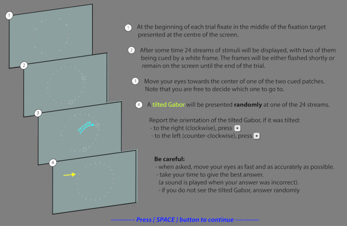
Figure 1: Instructions as presented to the participants. Visualization of the experimental instructions as presented to the participants at the beginning of each block. Please click here to view a larger version of this figure.
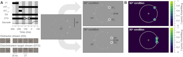
Figure 2: Experimental procedure and normalized saccade landing frequency maps. (A) Stimulus timing and display. Participants prepared a saccade from the fixation target (FT) to one of the two potential saccade targets (ST1 and ST2), presented simultaneously at two randomly chosen stimulus streams with an inter-target angular distance of either 90° (top panels) or 30° (bottom panels). The saccade targets were either shown continuously (cST1+2) or transiently (tST1+2). Stimulus streams could either be distractor streams (DS), composed of alternating vertical Gabors and masks (40 Hz) or discrimination target streams (DTS) which included the presentation of a brief discrimination target (DT, 25 ms), a clockwise or counterclockwise tilted Gabor, shown between 75 and 175 ms after the saccade targets onset. Participants saccaded towards one of the saccade targets and had to report the orientation of the discrimination target, appearing randomly at one of the 24 stimulus stream locations. Note that stimuli are sketched in order to increase their visibility. Actual stimuli match those shown in the stimulus streams depiction. (B) Normalized saccade landing frequency maps averaged across participants (n = 10) for the 90° (top) and 30° (bottom) conditions (collapsed across the transient and continuous ST presentation). This figure has been reprinted from Wollenberg et al. (2018)23. Please click here to view a larger version of this figure.
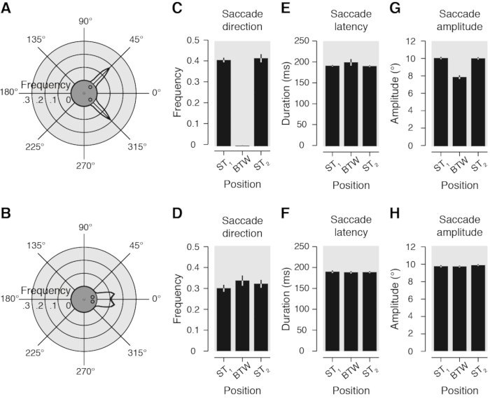
Figure 3: Saccade metrics. (A-B) Circular plots show the averaged frequency distribution of the saccade landing direction binned in evenly distributed angular sectors of 5°, in the 90° (A) and 30° conditions (B). Stimulus configuration is rotated as to align the two saccade targets symmetrically around the geometrical angle zero (see central insets). (C-D) Bar graphs illustrate averaged frequency of trials as a function of the saccade landing direction binned in 24 evenly distributed angular sectors of 15°. Data are shown for the three positions of interest (ST1, BTW and ST2) in the 90° (C) and 30° conditions (D). (E-H) Averaged saccade latency (E, F) and amplitude (G, H) observed for the same three positions of interest in the 90° (E, G) and 30° conditions (F, H). All data are shown irrespective of the duration (continuously or transiently) of the saccade targets. Light gray areas and error bars represent SEM. Polar plot black lines and corresponding light gray areas show linear interpolation between data points. This figure has been reprinted from Wollenberg et al. (2018)23. Please click here to view a larger version of this figure.
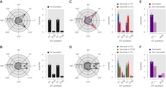
Figure 4: Visual sensitivity. (A-B). Circular plots show averaged visual sensitivity (d') as a function of the DT position in the 90° (A) and 30° conditions (B), irrespective of the duration of the saccade targets and across all saccade directions observed. Bar graphs illustrate visual sensitivity for four positions of interest (ST1, BTW, ST2, CTRL). (C-D) Visual sensitivity as a function of the DT position relative to the saccade landing direction in the 90° (C) and 30° conditions (D), irrespective of the duration of the saccade targets (blue: saccade to ST1; green: saccade to BTW; red: saccade to ST2). For each saccade direction, we took the average sensitivity for each discrimination target location. For example, the blue line plots visual sensitivity when saccades were made towards ST1 and the discrimination target was either at ST1 (+15° on the polar plot), BTW (15° counterclockwise to ST1; 0° on the polar plot) or ST2 (30° counterclockwise to ST1; + 345° on the polar plot), and so on. (E-F) Bar graphs illustrate sensitivity observed for DT shown at the saccaded (purple: e.g., DT at ST1 and saccade to ST1) and the non-saccaded positions (light-purple: e.g. DT at ST1 and saccade to ST2 or BTW) in the 90° (E) and the 30° (F) conditions. Conventions are as in Figure 3. This figure has been reprinted from Wollenberg et al. (2018)23. Please click here to view a larger version of this figure.

Figure 5: Corrective saccades. (A) Circular plot shows averaged frequency distribution of the corrective saccade landing direction following an averaging saccade. (B) The bar graph illustrates averaged frequency of trials as a function of the corrective saccade landing direction following an averaging saccade for three positions of interest (ST1, BTW and ST2). (C) The bar graph illustrates visual sensitivity as a function of the direction of the first corrective saccade for all trials in which an averaging saccade was executed. Purple bars show visual sensitivity for trials in which the corrective saccade was directed towards the location at which the DT appeared (e.g. DT at ST1 and corrective saccade towards ST1). Light purple bars show visual sensitivity for trials in which the corrective saccade was directed towards a different location than the location at which the DT appeared (e.g. DT at ST1 and corrective saccade towards ST2 or BTW). Conventions are as in Figure 3-4. This figure has been reprinted from Wollenberg et al. (2018)23. Please click here to view a larger version of this figure.
Discussion
This experimental protocol employed the concurrent assessment of gaze behavior and presaccadic visual sensitivity in a free choice saccade task. It allowed us to analyze whether visual attention is indeed obligatorily coupled to oculomotor programming at the behavioral level and therefore systematically deployed at the endpoint of saccades. Two saccade targets were presented in close proximity (30°) on half of the trials in which we observed a distinct global effect, reflected in a saccade landing distribution consisting of both, accurate and averaging saccades. To conclude on the spatial coupling between visual attention and the saccadic endpoint, visual sensitivity was analyzed and compared across different locations as a function of the saccade landing direction. While we observed a consistent and selective enhancement of visual sensitivity at the endpoint of accurate saccades, visual sensitivity was not enhanced at the endpoint of averaging saccades. Rather, visual sensitivity was equally facilitated at the two saccade targets before the execution of averaging saccades, suggesting that saccade averaging arises from unresolved attentional selection among the saccade targets. Our results, therefore, demonstrate that visual attention is not obligatorily deployed at the endpoint of the executed oculomotor program. A corrective saccade analysis, which demonstrated that the even deployment of visual sensitivity across the two saccade targets before averaging saccades did not systematically vary as a function the corrective saccade direction, further confirmed this interpretation. In this regard, our data are consistent with a recent model by Zirnsak et al.25 which assumes a target selection process that gradually builds up over time.
Importantly, our protocol differs from other behavioral studies that reported evidence for a dissociation between attention and saccades in several aspects. While some studies based their conclusion on saccadic reaction times14,15,16, we used a direct measure of visual spatial attention, namely visual sensitivity during saccade preparation. The specific parameters used throughout this protocol were effective in replicating the classical presaccadic shift of attention8,9 as evident in the consistent enhancement of visual sensitivity at the endpoint of accurate saccades. Thus, the protocol allowed for reliable detection of systematic modulations of visual attention specific to saccade preparation. This is an important prerequisite to validly interpret presaccadic attentional effects, and in particular, the observed absence of attentional enhancement at the endpoint of averaging saccades.
A central and distinct aspect of this protocol was the random presentation of the discrimination target among various locations. Thereby, we could sample visual sensitivity across the entire visual field, which consequently allowed us to not only determine whether attention is facilitated at the endpoint of saccades but also to investigate the spread of attention around this area including adjacent locations. The discrete allocation of attention at the two saccade targets (limited to less than ~2.6°, the distance between two of our adjacent stimuli) we observed before averaging saccades contradicts an early account which suggested that averaging saccades may reflect a coarse processing of the visual scene17 and argues for an enhancement of local rather than global visual information processing. Further, the random presentation of the discrimination target rendered its location completely unpredictable to participants. Thus, our protocol generally facilitated an even deployment of visual attention across the visual field with respect to the discrimination task. We consider this fact important with regard to any potential attentional effects and conclusions related to saccade preparation.
However, since eye movements are not typically performed while trying to discriminate stimuli across the entire visual field in natural vision, the results obtained in this protocol can not unrestrictedly account for oculomotor behavior in every day life. Furthermore, the oculomotor task did inevitably bias the deployment of attention via the saccade target cueing. The saccade targets did not only introduce relevant oculomotor goals but also salient exogenous cues that likely attracted attention. Thus, it is possible that visual discrimination performance at the intermediate location was generally deteriorated due to some masking elicited by the two surrounding saccade targets. In order to decrease the impact of the saccade targets with respect to discrimination performance at the intermediate location and to evaluate potential masking effects, we decided to present the saccade targets only transiently (for 50 ms) instead of continuously (until the trial end) on half of the trials. Consequently, even though both cueing conditions introduced visual onsets at the saccade target locations, the saccade targets had always disappeared before the onset of the discrimination target in the transient cueing condition. While the majority of results were very consistent across both cueing conditions and were therefore combined in the final analysis, we indeed observed an indication of a masking effect in the continuous cueing condition relative to the transient cueing condition. Overall, irrespective of the saccade direction, visual sensitivity at the intermediate location was slightly decreased in the continuous compared to the transient cueing condition. Given the notion that transient saccade target cueing apparently minimizes masking of the intermediate location while still being effective in eliciting averaging saccades, future studies using a protocol similar to ours should consider employing transient cueing of targets. However, despite our efforts to minimize masking effects via the transient cueing of targets, we can not rule out that the transient cueing still introduced a forward masking effect, which might potentially account for the poor discrimination performance at the intermediate location to some extent.
Taken together, our protocol allowed to directly address the coupling between visual attention and oculomotor programming, and to reveal a distinct spatial dissociation between attention and the endpoint of averaging saccades at the behavioral level. Our results argue against a mandatory coupling between visual attention and oculomotor programming suggested in the premotor theory of attention. Future studies should employ paradigms including concurrent neurophysiological recordings within areas such as the FEF and SC to further resolve the coupling between visual attention and oculomotor programming.
Disclosures
The authors have declared that no competing interests exist.
Acknowledgements
This research was supported by grants of the Deutsche Forschungsgemeinschaft to H.D. (DE336/5-1 and RTG 2175 "Perception in context and its neural basis") and to M.S. (SZ343/1) and a Marie Sklodowska-Curie Action Individual Fellowship to M.S. (704537).
Materials
| Name | Company | Catalog Number | Comments |
|---|---|---|---|
| Computer | Apple iMac (Cupertino, CA) | ||
| CRT Screen | Sony GDM F900 (Tokyo, Japan) | 24 inch screen with a spatial resolution of 1024 x 640 pixels and a vertical refresh rate of 120 Hz | |
| Eye Tracker | EyeLink 1000 Desktop Mount (SR Research, Osgoode, Ontario, Canada) | operating at a sampling rate of 1 kHz | |
| Software | Matlab (The MathWorks, Natick, MA) / toolboxes: Psychophics, EyeLink |
References
- Rizzolatti, G., Riggio, L., Dascola, I., Umiltá, C. Reorienting attention across the horizontal and vertical meridians: evidence in favor of a premotor theory of attention. Neuropsychologia. 25 (1), 31-40 (1997).
- Rizzolatti, G., Riggio, L., Sheliga, B. M. Space and selective attention. Attention and performance XV. 15, 231-265 (1994).
- Corbetta, M. Frontoparietal cortical networks for directing attention and the eye to visual locations: Identical, independent, or overlapping neural systems? Proceedings of the National Academy of Sciences. 95, 831-838 (1998).
- Müller, J. R., Philiastides, M. G., Newsome, W. T. Microstimulation of the superior colliculus focuses attention without moving the eyes. Proceedings of the National Academy of Sciences. 102 (3), 524-529 (2005).
- McPeek, R. M., Keller, E. L. Deficits in saccade target selection after inactivation of superior colliculus. Nature nueroscience. 7 (7), 757(2004).
- Moore, T., Armstrong, K. M. Selective gating of visual signals by microstimulation of frontal cortex. Nature. 421, 370(2003).
- Moore, T., Fallah, M. Microstimulation of the frontal eye field and its effects on covert spatial attention. Journal of neurophysiology. 91 (1), 152-162 (2004).
- Kowler, E., Anderson, E., Dosher, B., Blaser, E. The role of attention in the programming of saccades. Vision research. 35 (13), 1897-1916 (1995).
- Deubel, H., Schneider, W. X. Saccade target selection and object recognition: Evidence for a common attentional mechanism. Vision research. 36, 1827-1837 (1996).
- Thompson, K. G., Biscoe, K. L., Sato, T. R. Neuronal basis of covert spatial attention in the frontal eye field. Journal of Neuroscience. 25 (41), 9479-9487 (2005).
- Ignashchenkova, A., Dicke, P. W., Haarmeier, T., Thier, P. Neuron-specific contribution of the superior colliculus to overt and covert shifts of attention. Nature nueroscience. 7 (1), 56(2004).
- Gregoriou, G. G., Gotts, S. J., Desimone, R. Cell-type-specific synchronization of neural activity in FEF with V4 during attention. Neuron. 73 (3), 581-594 (2012).
- Born, S., Mottet, I., Kerzel, D. Presaccadic perceptual facilitation effects depend on saccade execution: Evidence from the stop-signal paradigm. Journal of Vision. 14 (3), 7-7 (2014).
- Belopolsky, A. V., Theeuwes, J. Updating the premotor theory: the allocation of attention is not always accompanied by saccade preparation. Journal of Experimental Psychology: Human Perception and Performance. 38 (4), 902(2012).
- Hunt, A. R., Kingstone, A. Covert and overt voluntary attention: linked or independent? Cognitive Brain Research. 18 (1), 102-105 (2003).
- Smith, D. T., Schenk, T., Rorden, C. Saccade preparation is required for exogenous attention but not endogenous attention or IOR. Journal of Experimental Psychology: Human Perception and Performance. 38 (6), 1438(2012).
- Findlay, J. M. Global visual processing for saccadic eye movements. Vision research. 22, 1033-1045 (1982).
- Coren, S., Hoenig, P. Effect of non-target stimuli upon length of voluntary saccades. Perceptual and motor skills. 34 (2), 499-508 (1972).
- Van der Stigchel, S., Nijboer, T. C. The global effect: what determines where the eyes land? Journal of Eye Movement Research. 4 (2), (2011).
- Vitu, F. About the global effect and the critical role of retinal eccentricity: Implications for eye movements in reading. Journal of Eye Movement Research. 2 (3), (2008).
- Hanning, N., Deubel, H., Szinte, M. Sensitivity measures of visuospatial attention. Journal of Vision. 17 (10), 673-673 (2017).
- Van der Stigchel, S., De Vries, J. P. There is no attentional global effect: Attentional shifts are independent of the saccade endpoint. Journal of vision. 15, 17-17 (2015).
- Wollenberg, L., Deubel, H., Szinte, M. Visual attention is not deployed at the endpoint of averaging saccades. PLoS biology. 16 (6), e2006548(2018).
- Engbert, R., Mergenthaler, K. Microsaccades are triggered by low retinal image slip. Proceedings of the National Academy of Sciences. 103 (18), 7192-7197 (2006).
- Zirnsak, M., Beuth, F., Hamker, F. H. Split of spatial attention as predicted by a systems-level model of visual attention. European Journal of Neuroscience. 33 (11), 2035-2045 (2011).
Reprints and Permissions
